This tutorial depends on step-7, step-9, step-61.
This program was contributed by Martin Kronbichler and Scott Miller.
Introduction
This tutorial program presents the implementation of a hybridizable discontinuous Galkerin method for the convection-diffusion equation.
Hybridizable discontinuous Galerkin methods
One common argument against the use of discontinuous Galerkin elements is the large number of globally coupled degrees of freedom that one must solve in an implicit system. This is because, unlike continuous finite elements, in typical discontinuous elements there is one degree of freedom at each vertex for each of the adjacent elements, rather than just one, and similarly for edges and faces. As an example of how fast the number of unknowns grows, consider the FE_DGPMonomial basis: each scalar solution component is represented by polynomials of degree \(p\) with \((1/\text{dim}!) \prod_{i=1}^{\text{dim}}(p+i)\) degrees of freedom per element. Typically, all degrees of freedom in an element are coupled to all of the degrees of freedom in the adjacent elements. The resulting discrete equations yield very large linear systems very quickly, especially for systems of equations in 2 or 3 dimensions.
Reducing the size of the linear system
To alleviate the computational cost of solving such large linear systems, the hybridizable discontinuous Galerkin (HDG) methodology was introduced by Cockburn and co-workers (see the references in the recent HDG overview article by Nguyen and Peraire [53]).
The HDG method achieves this goal by formulating the mathematical problem using Dirichlet-to-Neumann mappings. The partial differential equations are first written as a first order system, and each field is then discretized via a DG method. At this point, the single-valued "trace" values on the skeleton of the mesh, i.e., element faces, are taken to be independent unknown quantities. This yields unknowns in the discrete formulation that fall into two categories:
- Face unknowns that only couple with the cell unknowns from both sides of the face;
- Cell unknowns that only couple with the cell and face unknowns defined within the same cell. Crucially, no cell interior degree of freedom on one cell ever couples to any interior cell degree of freedom of a different cell.
The Dirichlet-to-Neumann map concept then permits the following solution procedure:
-
Use local element interior data to enforce a Neumann condition on the skeleton of the triangulation. The global problem is then to solve for the trace values, which are the only globally coupled unknowns.
-
Use the known skeleton values as Dirichlet data for solving local element-level solutions. This is known as the 'local solver', and is an embarrassingly parallel element-by-element solution process.
Relation with Static Condensation
The above procedure also has a linear algebra interpretation—referred to as static condensation—that was exploited to reduce the size of the global linear system by Guyan in the context of continuous Finite Elements [33], and by Fraeijs de Veubeke for mixed methods [26]. In the latter case (mixed formulation), the system reduction was achieved through the use of discontinuous fluxes combined with the introduction of an additional auxiliary hybrid variable that approximates the trace of the unknown at the boundary of every element. This procedure became known as hybridization and—by analogy—is the reason why the local discontinuous Galerkin method introduced by Cockburn, Gopalakrishnan, and Lazarov in 2009 [17], and subsequently developed by their collaborators, eventually came to be known as the hybridizable discontinuous Galerkin (HDG) method.
Let us write the complete linear system associated to the HDG problem as a block system with the discrete DG (cell interior) variables \(U\) as first block and the skeleton (face) variables \(\Lambda\) as the second block:
\begin{eqnarray*} \begin{pmatrix} A & B \\ C & D \end{pmatrix} \begin{pmatrix} U \\ \Lambda \end{pmatrix} = \begin{pmatrix} F \\ G \end{pmatrix}. \end{eqnarray*}
Our aim is now to eliminate the \(U\) block with a Schur complement approach similar to step-20, which results in the following two steps:
\begin{eqnarray*} (D - C A^{-1} B) \Lambda &=& G - C A^{-1} F, \\ A U &=& F - B \Lambda. \end{eqnarray*}
The point is that the presence of \(A^{-1}\) is not a problem because \(A\) is a block diagonal matrix where each block corresponds to one cell and is therefore easy enough to invert. The coupling to other cells is introduced by the matrices \(B\) and \(C\) over the skeleton variable. The block-diagonality of \(A\) and the structure in \(B\) and \(C\) allow us to invert the matrix \(A\) element by element (the local solution of the Dirichlet problem) and subtract \(CA^{-1}B\) from \(D\). The steps in the Dirichlet-to-Neumann map concept hence correspond to
-
constructing the Schur complement matrix \(D-C A^{-1} B\) and right hand side \(G - C A^{-1} F\) locally on each cell and inserting the contribution into the global trace matrix in the usual way,
-
solving the Schur complement system for \(\Lambda\), and
-
solving for \(U\) using the second equation, given \(\Lambda\).
Solution quality and rates of convergence
Another criticism of traditional DG methods is that the approximate fluxes converge suboptimally. The local HDG solutions can be shown to converge as \(\mathcal{O}(h^{p+1})\), i.e., at optimal order. Additionally, a super-convergence property can be used to post-process a new approximate solution that converges at the rate \(\mathcal{O}(h^{p+2})\).
Alternative approaches
The hybridizable discontinuous Galerkin method is only one way in which the problems of the discontinuous Galerkin method can be addressed. Another idea is what is called the "weak Galerkin" method. It is explored in step-61.
HDG applied to the convection-diffusion problem
The HDG formulation used for this example is taken from
N.C. Nguyen, J. Peraire, B. Cockburn: An implicit high-order hybridizable discontinuous Galerkin method for linear convection–diffusion equations, Journal of Computational Physics, 2009, 228:9, 3232-3254. [DOI]
We consider the convection-diffusion equation over the domain \(\Omega\) with Dirichlet boundary \(\partial \Omega_D\) and Neumann boundary \(\partial \Omega_N\):
\begin{eqnarray*} \nabla \cdot (\mathbf{c} u) - \nabla \cdot (\kappa \nabla u) &=& f, \quad \text{ in } \Omega, \\ u &=& g_D, \quad \text{ on } \partial \Omega_D, \\ (\mathbf{c} u - \kappa \nabla u)\cdot \mathbf{n} &=& g_N, \quad \text{ on } \partial \Omega_N. \end{eqnarray*}
Introduce the auxiliary variable \(\mathbf{q}=-\kappa \nabla u\) and rewrite the above equation as the first order system:
\begin{eqnarray*} \mathbf{q} + \kappa \nabla u &=& 0, \quad \text{ in } \Omega, \\ \nabla \cdot (\mathbf{c} u + \mathbf{q}) &=& f, \quad \text{ in } \Omega, \\ u &=& g_D, \quad \text{ on } \partial \Omega_D, \\ (\mathbf{q} + \mathbf{c}u)\cdot\mathbf{n} &=& g_N, \quad \text{ on } \partial \Omega_N. \end{eqnarray*}
We multiply these equations by the weight functions \(\mathbf{v}, w\) and integrate by parts over every element \(K\) to obtain:
\begin{eqnarray*} (\mathbf{v}, \kappa^{-1} \mathbf{q})_K - (\nabla\cdot\mathbf{v}, u)_K + \left<\mathbf{v}\cdot\mathbf{n}, {\hat{u}}\right>_{\partial K} &=& 0, \\ - (\nabla w, \mathbf{c} u + \mathbf{q})_K + \left<w, (\widehat{\mathbf{c} u}+{\hat{\mathbf{q}}})\cdot\mathbf{n}\right>_{\partial K} &=& (w,f)_K. \end{eqnarray*}
The terms decorated with a hat denote the numerical traces (also commonly referred to as numerical fluxes). They are approximations to the interior values on the boundary of the element. To ensure conservation, these terms must be single-valued on any given element edge \(\partial K\) even though, with discontinuous shape functions, there may of course be multiple values coming from the cells adjacent to an interface. We eliminate the numerical trace \(\hat{\mathbf{q}}\) by using traces of the form:
\begin{eqnarray*} \widehat{\mathbf{c} u}+\hat{\mathbf{q}} = \mathbf{c}\hat{u} + \mathbf{q} + \tau(u - \hat{u})\mathbf{n} \quad \text{ on } \partial K. \end{eqnarray*}
The variable \(\hat {u}\) is introduced as an additional independent variable and is the one for which we finally set up a globally coupled linear system. As mentioned above, it is defined on the element faces and discontinuous from one face to another wherever faces meet (at vertices in 2d, and at edges and vertices in 3d). Values for \(u\) and \(\mathbf{q}\) appearing in the numerical trace function are taken to be the cell's interior solution restricted to the boundary \(\partial K\).
The local stabilization parameter \(\tau\) has effects on stability and accuracy of HDG solutions; see the literature for a further discussion. A stabilization parameter of unity is reported to be the choice which gives best results. A stabilization parameter \(\tau\) that tends to infinity prohibits jumps in the solution over the element boundaries, making the HDG solution approach the approximation with continuous finite elements. In the program below, we choose the stabilization parameter as
\begin{eqnarray*} \tau = \frac{\kappa}{\ell} + |\mathbf{c} \cdot \mathbf{n}| \end{eqnarray*}
where we set the diffusion \(\kappa=1\) and the diffusion length scale to \(\ell = \frac{1}{5}\).
The trace/skeleton variables in HDG methods are single-valued on element faces. As such, they must strongly represent the Dirichlet data on \(\partial\Omega_D\). This means that
\begin{equation*} \hat{u}|_{\partial \Omega_D} = g_D, \end{equation*}
where the equal sign actually means an \(L_2\) projection of the boundary function \(g\) onto the space of the face variables (e.g. linear functions on the faces). This constraint is then applied to the skeleton variable \(\hat{u}\) using inhomogeneous constraints by the method VectorTools::project_boundary_values.
Summing the elemental contributions across all elements in the triangulation, enforcing the normal component of the numerical flux, and integrating by parts on the equation weighted by \(w\), we arrive at the final form of the problem: Find \((\mathbf{q}_h, u_h, \hat{u}_h) \in \mathcal{V}_h^p \times \mathcal{W}_h^p \times \mathcal{M}_h^p\) such that
\begin{align*} (\mathbf{v}, \kappa^{-1} \mathbf{q}_h)_{\mathcal{T}} - ( \nabla\cdot\mathbf{v}, u_h)_{\mathcal{T}} + \left<\mathbf{v}\cdot\mathbf{n}, \hat{u}_h\right>_{\partial\mathcal{T}} &= 0, \quad &&\forall \mathbf{v} \in \mathcal{V}_h^p, \\ - (\nabla w, \mathbf{c} u_h)_{\mathcal{T}} + (w, \nabla \cdot \mathbf{q}_h)_{\mathcal{T}} + (w, (\mathbf{c}\cdot\mathbf{n}) \hat{u}_h)_{\partial \mathcal{T}} + \left<w, \tau (u_h - \hat{u}_h)\right>_{\partial \mathcal{T}} &= (w, f)_{\mathcal{T}}, \quad &&\forall w \in \mathcal{W}_h^p, \\ \left< \mu, \hat{u}_h\mathbf{c} \cdot \mathbf{n} + \mathbf{q}_h\cdot \mathbf{n} + \tau (u_h - \hat{u}_h)\right>_{\partial \mathcal{T}} &= \left<\mu, g_N\right>_{\partial\Omega_N}, \quad &&\forall \mu \in \mathcal{M}_h^p. \end{align*}
The unknowns \((\mathbf{q}_h, u_h)\) are referred to as local variables; they are represented as standard DG variables. The unknown \(\hat{u}_h\) is the skeleton variable which has support on the codimension-1 surfaces (faces) of the mesh.
We use the notation \((\cdot, \cdot)_{\mathcal{T}} = \sum_K (\cdot, \cdot)_K\) to denote the sum of integrals over all cells and \(\left<\cdot, \cdot\right>_{\partial \mathcal{T}} = \sum_K \left<\cdot, \cdot\right>_{\partial K}\) to denote integration over all faces of all cells, i.e., interior faces are visited twice, once from each side and with the corresponding normal vectors. When combining the contribution from both elements sharing a face, the above equation yields terms familiar from the DG method, with jumps of the solution over the cell boundaries.
In the equation above, the space \(\mathcal {W}_h^{p}\) for the scalar variable \(u_h\) is defined as the space of functions that are tensor product polynomials of degree \(p\) on each cell and discontinuous over the element boundaries \(\mathcal Q_{-p}\), i.e., the space described by FE_DGQ<dim>(p). The space for the gradient or flux variable \(\mathbf{q}_i\) is a vector element space where each component is a locally polynomial and discontinuous \(\mathcal Q_{-p}\). In the code below, we collect these two local parts together in one FESystem where the first dim components denote the gradient part and the last scalar component corresponds to the scalar variable. For the skeleton component \(\hat{u}_h\), we define a space that consists of discontinuous tensor product polynomials that live on the element faces, which in deal.II is implemented by the class FE_FaceQ. This space is otherwise similar to FE_DGQ, i.e., the solution function is not continuous between two neighboring faces, see also the results section below for an illustration.
In the weak form given above, we can note the following coupling patterns:
-
The matrix \(A\) consists of local-local coupling terms. These arise when the local weighting functions \((\mathbf{v}, w)\) multiply the local solution terms \((\mathbf{q}_h, u_h)\). Because the elements are discontinuous, \(A\) is block diagonal.
-
The matrix \(B\) represents the local-face coupling. These are the terms with weighting functions \((\mathbf{v}, w)\) multiplying the skeleton variable \(\hat{u}_h\).
-
The matrix \(C\) represents the face-local coupling, which involves the weighting function \(\mu\) multiplying the local solutions \((\mathbf{q}_h, u_h)\).
-
The matrix \(D\) is the face-face coupling; terms involve both \(\mu\) and \(\hat{u}_h\).
Post-processing and super-convergence
One special feature of the HDG methods is that they typically allow for constructing an enriched solution that gains accuracy. This post-processing takes the HDG solution in an element-by-element fashion and combines it such that one can get \(\mathcal O(h^{p+2})\) order of accuracy when using polynomials of degree \(p\). For this to happen, there are two necessary ingredients:
-
The computed solution gradient \(\mathbf{q}_h\) converges at optimal rate, i.e., \(\mathcal{O}(h^{p+1})\).
-
The cell-wise average of the scalar part of the solution, \(\frac{(1,u_h)_K}{\text{vol}(K)}\), super-converges at rate \(\mathcal{O}(h^{p+2})\).
We now introduce a new variable \(u_h^* \in \mathcal{V}_h^{p+1}\), which we find by minimizing the expression \(|\kappa \nabla u_h^* + \mathbf{q}_h|^2\) over the cell \(K\) under the constraint \(\left(1, u_h^*\right)_K = \left(1, u_h\right)_K\). The constraint is necessary because the minimization functional does not determine the constant part of \(u_h^*\). This translates to the following system of equations:
\begin{eqnarray*} \left(1, u_h^*\right)_K &=& \left(1, u_h\right)_K\\ \left(\nabla w_h^*, \kappa \nabla u_h^*\right)_K &=& -\left(\nabla w_h^*, \mathbf{q}_h\right)_K \quad \text{for all } w_h^* \in \mathcal Q^{p+1}. \end{eqnarray*}
Since we test by the whole set of basis functions in the space of tensor product polynomials of degree \(p+1\) in the second set of equations, this is an overdetermined system with one more equation than unknowns. We fix this in the code below by omitting one of these equations (since the rows in the Laplacian are linearly dependent when representing a constant function). As we will see below, this form of the post-processing gives the desired super-convergence result with rate \(\mathcal {O}(h^{p+2})\). It should be noted that there is some freedom in constructing \(u_h^*\) and this minimization approach to extract the information from the gradient is not the only one. In particular, the post-processed solution defined here does not satisfy the convection-diffusion equation in any sense. As an alternative, the paper by Nguyen, Peraire and Cockburn cited above suggests another somewhat more involved formula for convection-diffusion that can also post-process the flux variable into an \(H(\Omega,\mathrm{div})\)-conforming variant and better represents the local convection-diffusion operator when the diffusion is small. We leave the implementation of a more sophisticated post-processing as a possible extension to the interested reader.
Note that for vector-valued problems, the post-processing works similarly. One simply sets the constraint for the mean value of each vector component separately and uses the gradient as the main source of information.
Problem specific data
For this tutorial program, we consider almost the same test case as in step-7. The computational domain is \(\Omega \dealcoloneq [-1,1]^d\) and the exact solution corresponds to the one in step-7, except for a scaling. We use the following source centers \(x_i\) for the exponentials
-
1D: \(\{x_i\}^1 = \{ -\frac{1}{3}, 0, \frac{1}{3} \}\),
-
2D: \(\{\mathbf{x}_i\}^2 = \{ (-\frac{1}{2},\frac{1}{2}), (-\frac{1}{2},-\frac{1}{2}), (\frac{1}{2},-\frac{1}{2}) \}\),
-
3D: \(\{\mathbf{x}_i\}^3 = \{ (-\frac{1}{2},\frac{1}{2}, \frac{1}{4}), (-\frac{3}{5},-\frac{1}{2}, -\frac{1}{8}), (\frac{1}{2},-\frac{1}{2}, \frac{1}{2}) \}\).
With the exact solution given, we then choose the forcing on the right hand side and the Neumann boundary condition such that we obtain this solution (manufactured solution technique). In this example, we choose the diffusion equal to one and the convection as
\[ \mathbf{c} = \begin{cases} 1, & \textrm{dim}=1 \\ (y, -x), & \textrm{dim}=2 \\ (y, -x, 1), & \textrm{dim}=3 \end{cases} \]
Note that the convection is divergence-free, \(\nabla \cdot c = 0\).
Implementation
Besides implementing the above equations, the implementation below provides the following features:
-
WorkStream to parallelize local solvers. Workstream has been presented in detail in step-9.
-
Reconstruct the local DG solution from the trace.
-
Post-processing the solution for superconvergence.
-
DataOutFaces for direct output of the global skeleton solution.
The commented program
Include files
Most of the deal.II include files have already been covered in previous examples and are not commented on.
However, we do have a few new includes for the example. The first one defines finite element spaces on the faces of the triangulation, which we refer to as the 'skeleton'. These finite elements do not have any support on the element interior, and they represent polynomials that have a single value on each codimension-1 surface, but admit discontinuities on codimension-2 surfaces.
The second new file we include defines a new type of sparse matrix. The regular SparseMatrix type stores indices to all non-zero entries. The ChunkSparseMatrix takes advantage of the coupled nature of DG solutions. It stores an index to a matrix sub-block of a specified size. In the HDG context, this sub-block-size is actually the number of degrees of freedom per face defined by the skeleton solution field. This reduces the memory consumption of the matrix by up to one third and results in similar speedups when using the matrix in solvers.
The final new include for this example deals with data output. Since we have a finite element field defined on the skeleton of the mesh, we would like to visualize what that solution actually is. DataOutFaces does exactly this; the interface is the almost the same as the familiar DataOut, but the output only has codimension-1 data for the simulation.
We start by putting all of our classes into their own namespace.
Equation data
The structure of the analytic solution is the same as in step-7. There are two exceptions. Firstly, we also create a solution for the 3d case, and secondly, we scale the solution so its norm is of order unity for all values of the solution width.
template <int dim>
class SolutionBase
{
protected:
static const unsigned int n_source_centers = 3;
static const Point<dim> source_centers[n_source_centers];
static const double width;
};
template <>
SolutionBase<1>::source_centers[SolutionBase<1>::n_source_centers] =
template <>
SolutionBase<2>::source_centers[SolutionBase<2>::n_source_centers] =
template <>
SolutionBase<3>::source_centers[SolutionBase<3>::n_source_centers] = {
template <int dim>
const double SolutionBase<dim>::width = 1. / 5.;
template <int dim>
class Solution :
public Function<dim>,
protected SolutionBase<dim>
{
public:
const unsigned int = 0) const override
{
for (unsigned int i = 0; i < this->n_source_centers; ++i)
{
}
}
const unsigned int = 0) const override
{
for (unsigned int i = 0; i < this->n_source_centers; ++i)
{
(-2 / (this->width * this->width) *
std::exp(-x_minus_xi.
norm_square() / (this->width * this->width)) *
x_minus_xi);
}
}
};
This class implements a function where the scalar solution and its negative gradient are collected together. This function is used when computing the error of the HDG approximation and its implementation is to simply call value and gradient function of the Solution class.
template <int dim>
class SolutionAndGradient :
public Function<dim>,
protected SolutionBase<dim>
{
public:
SolutionAndGradient()
{}
{
Solution<dim> solution;
for (
unsigned int d = 0;
d < dim; ++
d)
v[dim] = solution.value(p);
}
};
Next comes the implementation of the convection velocity. As described in the introduction, we choose a velocity field that is \((y, -x)\) in 2D and \((y, -x, 1)\) in 3D. This gives a divergence-free velocity field.
template <int dim>
{
public:
ConvectionVelocity()
{}
{
switch (dim)
{
case 1:
convection[0] = 1;
break;
case 2:
convection[0] = p[1];
convection[1] = -p[0];
break;
case 3:
convection[0] = p[1];
convection[1] = -p[0];
convection[2] = 1;
break;
default:
}
return convection;
}
};
The last function we implement is the right hand side for the manufactured solution. It is very similar to step-7, with the exception that we now have a convection term instead of the reaction term. Since the velocity field is incompressible, i.e., \(\nabla \cdot \mathbf{c} = 0\), the advection term simply reads \(\mathbf{c} \nabla u\).
template <int dim>
class RightHandSide :
public Function<dim>,
protected SolutionBase<dim>
{
public:
const unsigned int = 0) const override
{
ConvectionVelocity<dim> convection_velocity;
for (unsigned int i = 0; i < this->n_source_centers; ++i)
{
((2 * dim - 2 * convection * x_minus_xi -
4 * x_minus_xi.
norm_square() / (this->width * this->width)) /
(this->width * this->width) *
std::exp(-x_minus_xi.
norm_square() / (this->width * this->width)));
}
}
};
The HDG solver class
The HDG solution procedure follows closely that of step-7. The major difference is the use of three different sets of DoFHandler and FE objects, along with the ChunkSparseMatrix and the corresponding solutions vectors. We also use WorkStream to enable a multithreaded local solution process which exploits the embarrassingly parallel nature of the local solver. For WorkStream, we define the local operations on a cell and a copy function into the global matrix and vector. We do this both for the assembly (which is run twice, once when we generate the system matrix and once when we compute the element-interior solutions from the skeleton values) and for the postprocessing where we extract a solution that converges at higher order.
template <int dim>
class HDG
{
public:
enum RefinementMode
{
global_refinement,
adaptive_refinement
};
HDG(const unsigned int degree, const RefinementMode refinement_mode);
private:
void setup_system();
void assemble_system(const bool reconstruct_trace = false);
void solve();
void postprocess();
void refine_grid(const unsigned int cycle);
void output_results(const unsigned int cycle);
Data for the assembly and solution of the primal variables.
struct PerTaskData;
struct ScratchData;
Post-processing the solution to obtain \(u^*\) is an element-by-element procedure; as such, we do not need to assemble any global data and do not declare any 'task data' for WorkStream to use.
struct PostProcessScratchData;
The following three functions are used by WorkStream to do the actual work of the program.
void assemble_system_one_cell(
ScratchData & scratch,
PerTaskData & task_data);
void copy_local_to_global(const PerTaskData &data);
void postprocess_one_cell(
PostProcessScratchData & scratch,
unsigned int & empty_data);
The 'local' solutions are interior to each element. These represent the primal solution field \(u\) as well as the auxiliary field \(\mathbf{q}\).
The new finite element type and corresponding DoFHandler are used for the global skeleton solution that couples the element-level local solutions.
As stated in the introduction, HDG solutions can be post-processed to attain superconvergence rates of \(\mathcal{O}(h^{p+2})\). The post-processed solution is a discontinuous finite element solution representing the primal variable on the interior of each cell. We define a FE type of degree \(p+1\) to represent this post-processed solution, which we only use for output after constructing it.
The degrees of freedom corresponding to the skeleton strongly enforce Dirichlet boundary conditions, just as in a continuous Galerkin finite element method. We can enforce the boundary conditions in an analogous manner via an AffineConstraints object. In addition, hanging nodes are handled in the same way as for continuous finite elements: For the face elements which only define degrees of freedom on the face, this process sets the solution on the refined side to coincide with the representation on the coarse side.
Note that for HDG, the elimination of hanging nodes is not the only possibility — in terms of the HDG theory, one could also use the unknowns from the refined side and express the local solution on the coarse side through the trace values on the refined side. However, such a setup is not as easily implemented in terms of deal.II loops and not further analyzed.
The usage of the ChunkSparseMatrix class is similar to the usual sparse matrices: You need a sparsity pattern of type ChunkSparsityPattern and the actual matrix object. When creating the sparsity pattern, we just have to additionally pass the size of local blocks.
Same as step-7:
const RefinementMode refinement_mode;
};
The HDG class implementation
Constructor
The constructor is similar to those in other examples, with the exception of handling multiple DoFHandler and FiniteElement objects. Note that we create a system of finite elements for the local DG part, including the gradient/flux part and the scalar part.
template <int dim>
HDG<dim>::HDG(const unsigned int degree, const RefinementMode refinement_mode)
: fe_local(
FE_DGQ<dim>(degree), dim,
FE_DGQ<dim>(degree), 1)
, fe(degree)
, fe_u_post(degree + 1)
, refinement_mode(refinement_mode)
{}
HDG::setup_system
The system for an HDG solution is setup in an analogous manner to most of the other tutorial programs. We are careful to distribute dofs with all of our DoFHandler objects. The solution and system_matrix objects go with the global skeleton solution.
template <int dim>
void HDG<dim>::setup_system()
{
dof_handler_local.distribute_dofs(fe_local);
dof_handler_u_post.distribute_dofs(fe_u_post);
std::cout <<
" Number of degrees of freedom: " << dof_handler.
n_dofs()
<< std::endl;
solution.reinit(dof_handler.
n_dofs());
solution_local.reinit(dof_handler_local.n_dofs());
solution_u_post.reinit(dof_handler_u_post.n_dofs());
constraints.clear();
std::map<types::boundary_id, const Function<dim> *> boundary_functions;
Solution<dim> solution_function;
boundary_functions[0] = &solution_function;
boundary_functions,
constraints);
constraints.close();
When creating the chunk sparsity pattern, we first create the usual dynamic sparsity pattern and then set the chunk size, which is equal to the number of dofs on a face, when copying this into the final sparsity pattern.
{
sparsity_pattern.
copy_from(dsp, fe.dofs_per_face);
}
system_matrix.reinit(sparsity_pattern);
}
HDG::PerTaskData
Next comes the definition of the local data structures for the parallel assembly. The first structure PerTaskData contains the local vector and matrix that are written into the global matrix, whereas the ScratchData contains all data that we need for the local assembly. There is one variable worth noting here, namely the boolean variable trace_reconstruct. As mentioned in the introduction, we solve the HDG system in two steps. First, we create a linear system for the skeleton system where we condense the local part into it via the Schur complement \(D-CA^{-1}B\). Then, we solve for the local part using the skeleton solution. For these two steps, we need the same matrices on the elements twice, which we want to compute by two assembly steps. Since most of the code is similar, we do this with the same function but only switch between the two based on a flag that we set when starting the assembly. Since we need to pass this information on to the local worker routines, we store it once in the task data.
template <int dim>
struct HDG<dim>::PerTaskData
{
std::vector<types::global_dof_index> dof_indices;
bool trace_reconstruct;
PerTaskData(const unsigned int n_dofs, const bool trace_reconstruct)
, cell_vector(n_dofs)
, dof_indices(n_dofs)
, trace_reconstruct(trace_reconstruct)
{}
};
HDG::ScratchData
ScratchData contains persistent data for each thread within WorkStream. The FEValues, matrix, and vector objects should be familiar by now. There are two objects that need to be discussed: std::vector<std::vector<unsigned int> > fe_local_support_on_face and std::vector<std::vector<unsigned int> > fe_support_on_face. These are used to indicate whether or not the finite elements chosen have support (non-zero values) on a given face of the reference cell for the local part associated to fe_local and the skeleton part fe. We extract this information in the constructor and store it once for all cells that we work on. Had we not stored this information, we would be forced to assemble a large number of zero terms on each cell, which would significantly slow the program.
template <int dim>
struct HDG<dim>::ScratchData
{
std::vector<Tensor<1, dim>> q_phi;
std::vector<double> q_phi_div;
std::vector<double> u_phi;
std::vector<Tensor<1, dim>> u_phi_grad;
std::vector<double> tr_phi;
std::vector<double> trace_values;
std::vector<std::vector<unsigned int>> fe_local_support_on_face;
std::vector<std::vector<unsigned int>> fe_support_on_face;
ConvectionVelocity<dim> convection_velocity;
RightHandSide<dim> right_hand_side;
const Solution<dim> exact_solution;
: fe_values_local(fe_local, quadrature_formula, local_flags)
, fe_face_values_local(fe_local,
face_quadrature_formula,
local_face_flags)
, fe_face_values(fe, face_quadrature_formula, flags)
, ll_matrix(fe_local.dofs_per_cell, fe_local.dofs_per_cell)
, lf_matrix(fe_local.dofs_per_cell, fe.dofs_per_cell)
, fl_matrix(fe.dofs_per_cell, fe_local.dofs_per_cell)
, tmp_matrix(fe.dofs_per_cell, fe_local.dofs_per_cell)
, l_rhs(fe_local.dofs_per_cell)
, tmp_rhs(fe_local.dofs_per_cell)
, q_phi(fe_local.dofs_per_cell)
, q_phi_div(fe_local.dofs_per_cell)
, u_phi(fe_local.dofs_per_cell)
, u_phi_grad(fe_local.dofs_per_cell)
, tr_phi(fe.dofs_per_cell)
, trace_values(face_quadrature_formula.size())
, fe_local_support_on_face(
GeometryInfo<dim>::faces_per_cell)
, exact_solution()
{
{
fe_local_support_on_face[face_no].push_back(i);
}
{
fe_support_on_face[face_no].push_back(i);
}
}
ScratchData(const ScratchData &sd)
: fe_values_local(sd.fe_values_local.get_fe(),
sd.fe_values_local.get_quadrature(),
sd.fe_values_local.get_update_flags())
, fe_face_values_local(sd.fe_face_values_local.get_fe(),
sd.fe_face_values_local.get_quadrature(),
sd.fe_face_values_local.get_update_flags())
, fe_face_values(sd.fe_face_values.get_fe(),
sd.fe_face_values.get_quadrature(),
sd.fe_face_values.get_update_flags())
, ll_matrix(sd.ll_matrix)
, lf_matrix(sd.lf_matrix)
, fl_matrix(sd.fl_matrix)
, tmp_matrix(sd.tmp_matrix)
, l_rhs(sd.l_rhs)
, tmp_rhs(sd.tmp_rhs)
, q_phi(sd.q_phi)
, q_phi_div(sd.q_phi_div)
, u_phi(sd.u_phi)
, u_phi_grad(sd.u_phi_grad)
, tr_phi(sd.tr_phi)
, trace_values(sd.trace_values)
, fe_local_support_on_face(sd.fe_local_support_on_face)
, fe_support_on_face(sd.fe_support_on_face)
, exact_solution()
{}
};
HDG::PostProcessScratchData
PostProcessScratchData contains the data used by WorkStream when post-processing the local solution \(u^*\). It is similar, but much simpler, than ScratchData.
template <int dim>
struct HDG<dim>::PostProcessScratchData
{
std::vector<double> u_values;
std::vector<Tensor<1, dim>> u_gradients;
: fe_values_local(fe_local, quadrature_formula, local_flags)
, fe_values(fe, quadrature_formula, flags)
, u_values(quadrature_formula.size())
, u_gradients(quadrature_formula.size())
, cell_rhs(fe.dofs_per_cell)
, cell_sol(fe.dofs_per_cell)
{}
PostProcessScratchData(const PostProcessScratchData &sd)
: fe_values_local(sd.fe_values_local.get_fe(),
sd.fe_values_local.get_quadrature(),
sd.fe_values_local.get_update_flags())
, fe_values(sd.fe_values.get_fe(),
sd.fe_values.get_quadrature(),
sd.fe_values.get_update_flags())
, u_values(sd.u_values)
, u_gradients(sd.u_gradients)
, cell_rhs(sd.cell_rhs)
, cell_sol(sd.cell_sol)
{}
};
HDG::assemble_system
The assemble_system function is similar to the one on step-32, where the quadrature formula and the update flags are set up, and then WorkStream is used to do the work in a multi-threaded manner. The trace_reconstruct input parameter is used to decide whether we are solving for the global skeleton solution (false) or the local solution (true).
One thing worth noting for the multi-threaded execution of assembly is the fact that the local computations in assemble_system_one_cell() call into BLAS and LAPACK functions if those are available in deal.II. Thus, the underlying BLAS/LAPACK library must support calls from multiple threads at the same time. Most implementations do support this, but some libraries need to be built in a specific way to avoid problems. For example, OpenBLAS compiled without multithreading inside the BLAS/LAPACK calls needs to built with a flag called USE_LOCKING set to true.
template <int dim>
void HDG<dim>::assemble_system(const bool trace_reconstruct)
{
const QGauss<dim - 1> face_quadrature_formula(fe.
degree + 1);
ScratchData scratch(fe,
fe_local,
quadrature_formula,
face_quadrature_formula,
local_flags,
local_face_flags,
flags);
*this,
&HDG<dim>::assemble_system_one_cell,
&HDG<dim>::copy_local_to_global,
scratch,
task_data);
}
HDG::assemble_system_one_cell
The real work of the HDG program is done by assemble_system_one_cell. Assembling the local matrices \(A, B, C\) is done here, along with the local contributions of the global matrix \(D\).
template <int dim>
void HDG<dim>::assemble_system_one_cell(
ScratchData & scratch,
PerTaskData & task_data)
{
Construct iterator for dof_handler_local for FEValues reinit function.
cell->level(),
cell->index(),
&dof_handler_local);
const unsigned int n_q_points =
scratch.fe_values_local.get_quadrature().size();
const unsigned int n_face_q_points =
scratch.fe_face_values_local.get_quadrature().size();
const unsigned int loc_dofs_per_cell =
scratch.fe_values_local.get_fe().dofs_per_cell;
scratch.ll_matrix = 0;
scratch.l_rhs = 0;
if (!task_data.trace_reconstruct)
{
scratch.lf_matrix = 0;
scratch.fl_matrix = 0;
task_data.cell_matrix = 0;
task_data.cell_vector = 0;
}
scratch.fe_values_local.reinit(loc_cell);
We first compute the cell-interior contribution to ll_matrix matrix (referred to as matrix \(A\) in the introduction) corresponding to local-local coupling, as well as the local right-hand-side vector. We store the values at each quadrature point for the basis functions, the right-hand-side value, and the convection velocity, in order to have quick access to these fields.
for (unsigned int q = 0; q < n_q_points; ++q)
{
const double rhs_value = scratch.right_hand_side.value(
scratch.fe_values_local.quadrature_point(q));
scratch.fe_values_local.quadrature_point(q));
const double JxW = scratch.fe_values_local.JxW(q);
for (unsigned int k = 0; k < loc_dofs_per_cell; ++k)
{
scratch.q_phi[k] = scratch.fe_values_local[fluxes].value(k, q);
scratch.q_phi_div[k] =
scratch.fe_values_local[fluxes].divergence(k, q);
scratch.u_phi[k] = scratch.fe_values_local[scalar].value(k, q);
scratch.u_phi_grad[k] =
scratch.fe_values_local[scalar].gradient(k, q);
}
for (unsigned int i = 0; i < loc_dofs_per_cell; ++i)
{
for (unsigned int j = 0; j < loc_dofs_per_cell; ++j)
scratch.ll_matrix(i, j) +=
(scratch.q_phi[i] * scratch.q_phi[j] -
scratch.q_phi_div[i] * scratch.u_phi[j] +
scratch.u_phi[i] * scratch.q_phi_div[j] -
(scratch.u_phi_grad[i] * convection) * scratch.u_phi[j]) *
JxW;
scratch.l_rhs(i) += scratch.u_phi[i] * rhs_value * JxW;
}
}
Face terms are assembled on all faces of all elements. This is in contrast to more traditional DG methods, where each face is only visited once in the assembly procedure.
{
scratch.fe_face_values_local.reinit(loc_cell, face_no);
scratch.fe_face_values.reinit(cell, face_no);
The already obtained \(\hat{u}\) values are needed when solving for the local variables.
if (task_data.trace_reconstruct)
scratch.fe_face_values.get_function_values(solution,
scratch.trace_values);
for (unsigned int q = 0; q < n_face_q_points; ++q)
{
const double JxW = scratch.fe_face_values.JxW(q);
scratch.fe_face_values.quadrature_point(q);
scratch.fe_face_values.normal_vector(q);
scratch.convection_velocity.value(quadrature_point);
Here we compute the stabilization parameter discussed in the introduction: since the diffusion is one and the diffusion length scale is set to 1/5, it simply results in a contribution of 5 for the diffusion part and the magnitude of convection through the element boundary in a centered scheme for the convection part.
const double tau_stab = (5. +
std::abs(convection * normal));
We store the non-zero flux and scalar values, making use of the support_on_face information we created in ScratchData.
for (unsigned int k = 0;
k < scratch.fe_local_support_on_face[face_no].size();
++k)
{
const unsigned int kk =
scratch.fe_local_support_on_face[face_no][k];
scratch.q_phi[k] =
scratch.fe_face_values_local[fluxes].value(kk, q);
scratch.u_phi[k] =
scratch.fe_face_values_local[scalar].value(kk, q);
}
When trace_reconstruct=false, we are preparing to assemble the system for the skeleton variable \(\hat{u}\). If this is the case, we must assemble all local matrices associated with the problem: local-local, local-face, face-local, and face-face. The face-face matrix is stored as TaskData::cell_matrix, so that it can be assembled into the global system by copy_local_to_global.
if (!task_data.trace_reconstruct)
{
for (unsigned int k = 0;
k < scratch.fe_support_on_face[face_no].size();
++k)
scratch.tr_phi[k] = scratch.fe_face_values.shape_value(
scratch.fe_support_on_face[face_no][k], q);
for (unsigned int i = 0;
i < scratch.fe_local_support_on_face[face_no].size();
++i)
for (unsigned int j = 0;
j < scratch.fe_support_on_face[face_no].size();
++j)
{
const unsigned int ii =
scratch.fe_local_support_on_face[face_no][i];
const unsigned int jj =
scratch.fe_support_on_face[face_no][j];
scratch.lf_matrix(ii, jj) +=
((scratch.q_phi[i] * normal +
(convection * normal - tau_stab) * scratch.u_phi[i]) *
scratch.tr_phi[j]) *
JxW;
Note the sign of the face_no-local matrix. We negate the sign during assembly here so that we can use the FullMatrix::mmult with addition when computing the Schur complement.
scratch.fl_matrix(jj, ii) -=
((scratch.q_phi[i] * normal +
tau_stab * scratch.u_phi[i]) *
scratch.tr_phi[j]) *
JxW;
}
for (unsigned int i = 0;
i < scratch.fe_support_on_face[face_no].size();
++i)
for (unsigned int j = 0;
j < scratch.fe_support_on_face[face_no].size();
++j)
{
const unsigned int ii =
scratch.fe_support_on_face[face_no][i];
const unsigned int jj =
scratch.fe_support_on_face[face_no][j];
task_data.cell_matrix(ii, jj) +=
((convection * normal - tau_stab) * scratch.tr_phi[i] *
scratch.tr_phi[j]) *
JxW;
}
if (cell->face(face_no)->at_boundary() &&
(cell->face(face_no)->boundary_id() == 1))
{
const double neumann_value =
-scratch.exact_solution.gradient(quadrature_point) *
normal +
convection * normal *
scratch.exact_solution.value(quadrature_point);
for (unsigned int i = 0;
i < scratch.fe_support_on_face[face_no].size();
++i)
{
const unsigned int ii =
scratch.fe_support_on_face[face_no][i];
task_data.cell_vector(ii) +=
scratch.tr_phi[i] * neumann_value * JxW;
}
}
}
This last term adds the contribution of the term \(\left<w,\tau u_h\right>_{\partial \mathcal T}\) to the local matrix. As opposed to the face matrices above, we need it in both assembly stages.
for (unsigned int i = 0;
i < scratch.fe_local_support_on_face[face_no].size();
++i)
for (unsigned int j = 0;
j < scratch.fe_local_support_on_face[face_no].size();
++j)
{
const unsigned int ii =
scratch.fe_local_support_on_face[face_no][i];
const unsigned int jj =
scratch.fe_local_support_on_face[face_no][j];
scratch.ll_matrix(ii, jj) +=
tau_stab * scratch.u_phi[i] * scratch.u_phi[j] * JxW;
}
When trace_reconstruct=true, we are solving for the local solutions on an element by element basis. The local right-hand-side is calculated by replacing the basis functions tr_phi in the lf_matrix computation by the computed values trace_values. Of course, the sign of the matrix is now minus since we have moved everything to the other side of the equation.
if (task_data.trace_reconstruct)
for (unsigned int i = 0;
i < scratch.fe_local_support_on_face[face_no].size();
++i)
{
const unsigned int ii =
scratch.fe_local_support_on_face[face_no][i];
scratch.l_rhs(ii) -=
(scratch.q_phi[i] * normal +
scratch.u_phi[i] * (convection * normal - tau_stab)) *
scratch.trace_values[q] * JxW;
}
}
}
Once assembly of all of the local contributions is complete, we must either: (1) assemble the global system, or (2) compute the local solution values and save them. In either case, the first step is to invert the local-local matrix.
scratch.ll_matrix.gauss_jordan();
For (1), we compute the Schur complement and add it to the cell_matrix, matrix \(D\) in the introduction.
if (task_data.trace_reconstruct == false)
{
scratch.fl_matrix.mmult(scratch.tmp_matrix, scratch.ll_matrix);
scratch.tmp_matrix.vmult_add(task_data.cell_vector, scratch.l_rhs);
scratch.tmp_matrix.mmult(task_data.cell_matrix,
scratch.lf_matrix,
true);
cell->get_dof_indices(task_data.dof_indices);
}
For (2), we are simply solving (ll_matrix).(solution_local) = (l_rhs). Hence, we multiply l_rhs by our already inverted local-local matrix and store the result using the set_dof_values function.
else
{
scratch.ll_matrix.vmult(scratch.tmp_rhs, scratch.l_rhs);
loc_cell->set_dof_values(scratch.tmp_rhs, solution_local);
}
}
HDG::copy_local_to_global
If we are in the first step of the solution, i.e. trace_reconstruct=false, then we assemble the local matrices into the global system.
template <int dim>
void HDG<dim>::copy_local_to_global(const PerTaskData &data)
{
if (data.trace_reconstruct == false)
constraints.distribute_local_to_global(data.cell_matrix,
data.cell_vector,
data.dof_indices,
system_matrix,
system_rhs);
}
HDG::solve
The skeleton solution is solved for by using a BiCGStab solver with identity preconditioner.
template <int dim>
void HDG<dim>::solve()
{
std::cout << " Number of BiCGStab iterations: "
<< solver_control.last_step() << std::endl;
system_matrix.clear();
sparsity_pattern.
reinit(0, 0, 0, 1);
constraints.distribute(solution);
Once we have solved for the skeleton solution, we can solve for the local solutions in an element-by-element fashion. We do this by re-using the same assemble_system function but switching trace_reconstruct to true.
HDG::postprocess
The postprocess method serves two purposes. First, we want to construct a post-processed scalar variables in the element space of degree \(p+1\) that we hope will converge at order \(p+2\). This is again an element-by-element process and only involves the scalar solution as well as the gradient on the local cell. To do this, we introduce the already defined scratch data together with some update flags and run the work stream to do this in parallel.
Secondly, we want to compute discretization errors just as we did in step-7. The overall procedure is similar with calls to VectorTools::integrate_difference. The difference is in how we compute the errors for the scalar variable and the gradient variable. In step-7, we did this by computing L2_norm or H1_seminorm contributions. Here, we have a DoFHandler with these two contributions computed and sorted by their vector component, [0, dim) for the gradient and dim for the scalar. To compute their value, we hence use a ComponentSelectFunction with either of them, together with the SolutionAndGradient class introduced above that contains the analytic parts of either of them. Eventually, we also compute the L2-error of the post-processed solution and add the results into the convergence table.
template <int dim>
void HDG<dim>::postprocess()
{
{
const QGauss<dim> quadrature_formula(fe_u_post.degree + 1);
PostProcessScratchData scratch(
fe_u_post, fe_local, quadrature_formula, local_flags, flags);
dof_handler_u_post.begin_active(),
dof_handler_u_post.end(),
PostProcessScratchData & scratch,
unsigned int & data) {
this->postprocess_one_cell(cell, scratch, data);
},
std::function<void(const unsigned int &)>(),
scratch,
}
solution_local,
SolutionAndGradient<dim>(),
difference_per_cell,
&value_select);
const double L2_error =
difference_per_cell,
std::pair<unsigned int, unsigned int>(0, dim), dim + 1);
solution_local,
SolutionAndGradient<dim>(),
difference_per_cell,
&gradient_select);
const double grad_error =
difference_per_cell,
solution_u_post,
Solution<dim>(),
difference_per_cell,
const double post_error =
difference_per_cell,
convergence_table.add_value(
"cells",
triangulation.n_active_cells());
convergence_table.add_value(
"dofs", dof_handler.
n_dofs());
convergence_table.add_value("val L2", L2_error);
convergence_table.set_scientific("val L2", true);
convergence_table.set_precision("val L2", 3);
convergence_table.add_value("grad L2", grad_error);
convergence_table.set_scientific("grad L2", true);
convergence_table.set_precision("grad L2", 3);
convergence_table.add_value("val L2-post", post_error);
convergence_table.set_scientific("val L2-post", true);
convergence_table.set_precision("val L2-post", 3);
}
HDG::postprocess_one_cell
This is the actual work done for the postprocessing. According to the discussion in the introduction, we need to set up a system that projects the gradient part of the DG solution onto the gradient of the post-processed variable. Moreover, we need to set the average of the new post-processed variable to equal the average of the scalar DG solution on the cell.
More technically speaking, the projection of the gradient is a system that would potentially fills our dofs_per_cell times dofs_per_cell matrix but is singular (the sum of all rows would be zero because the constant function has zero gradient). Therefore, we take one row away and use it for imposing the average of the scalar value. We pick the first row for the scalar part, even though we could pick any row for \(\mathcal Q_{-p}\) elements. However, had we used FE_DGP elements instead, the first row would correspond to the constant part already and deleting e.g. the last row would give us a singular system. This way, our program can also be used for those elements.
template <int dim>
void HDG<dim>::postprocess_one_cell(
PostProcessScratchData & scratch,
unsigned int &)
{
cell->level(),
cell->index(),
&dof_handler_local);
scratch.fe_values_local.reinit(loc_cell);
scratch.fe_values.reinit(cell);
const unsigned int n_q_points = scratch.fe_values.get_quadrature().size();
const unsigned int dofs_per_cell = scratch.fe_values.dofs_per_cell;
scratch.fe_values_local[scalar].get_function_values(solution_local,
scratch.u_values);
scratch.fe_values_local[fluxes].get_function_values(solution_local,
scratch.u_gradients);
for (unsigned int i = 1; i < dofs_per_cell; ++i)
{
for (unsigned int j = 0; j < dofs_per_cell; ++j)
{
for (unsigned int q = 0; q < n_q_points; ++q)
sum += (scratch.fe_values.shape_grad(i, q) *
scratch.fe_values.shape_grad(j, q)) *
scratch.fe_values.JxW(q);
scratch.cell_matrix(i, j) =
sum;
}
for (unsigned int q = 0; q < n_q_points; ++q)
sum -= (scratch.fe_values.shape_grad(i, q) * scratch.u_gradients[q]) *
scratch.fe_values.JxW(q);
scratch.cell_rhs(i) =
sum;
}
for (unsigned int j = 0; j < dofs_per_cell; ++j)
{
for (unsigned int q = 0; q < n_q_points; ++q)
sum += scratch.fe_values.shape_value(j, q) * scratch.fe_values.JxW(q);
scratch.cell_matrix(0, j) =
sum;
}
{
for (unsigned int q = 0; q < n_q_points; ++q)
sum += scratch.u_values[q] * scratch.fe_values.JxW(q);
scratch.cell_rhs(0) =
sum;
}
Having assembled all terms, we can again go on and solve the linear system. We invert the matrix and then multiply the inverse by the right hand side. An alternative (and more numerically stable) method would have been to only factorize the matrix and apply the factorization.
scratch.cell_matrix.gauss_jordan();
scratch.cell_matrix.vmult(scratch.cell_sol, scratch.cell_rhs);
cell->distribute_local_to_global(scratch.cell_sol, solution_u_post);
}
HDG::output_results
We have 3 sets of results that we would like to output: the local solution, the post-processed local solution, and the skeleton solution. The former 2 both 'live' on element volumes, whereas the latter lives on codimension-1 surfaces of the triangulation. Our output_results function writes all local solutions to the same vtk file, even though they correspond to different DoFHandler objects. The graphical output for the skeleton variable is done through use of the DataOutFaces class.
template <int dim>
void HDG<dim>::output_results(const unsigned int cycle)
{
std::string filename;
switch (refinement_mode)
{
case global_refinement:
filename = "solution-global";
break;
case adaptive_refinement:
filename = "solution-adaptive";
break;
default:
}
std::string face_out(filename);
face_out += "-face";
filename += ".vtk";
std::ofstream output(filename);
We first define the names and types of the local solution, and add the data to data_out.
std::vector<std::string> names(dim, "gradient");
names.emplace_back("solution");
std::vector<DataComponentInterpretation::DataComponentInterpretation>
component_interpretation(
component_interpretation[dim] =
solution_local,
names,
component_interpretation);
The second data item we add is the post-processed solution. In this case, it is a single scalar variable belonging to a different DoFHandler.
std::vector<std::string> post_name(1, "u_post");
std::vector<DataComponentInterpretation::DataComponentInterpretation>
solution_u_post,
post_name,
post_comp_type);
face_out += ".vtk";
std::ofstream face_output(face_out);
The DataOutFaces class works analogously to the DataOut class when we have a DoFHandler that defines the solution on the skeleton of the triangulation. We treat it as such here, and the code is similar to that above.
std::vector<std::string> face_name(1, "u_hat");
std::vector<DataComponentInterpretation::DataComponentInterpretation>
data_out_face.add_data_vector(dof_handler,
solution,
face_name,
face_component_type);
data_out_face.build_patches(fe.
degree);
data_out_face.write_vtk(face_output);
}
HDG::refine_grid
We implement two different refinement cases for HDG, just as in step-7: adaptive_refinement and global_refinement. The global_refinement option recreates the entire triangulation every time. This is because we want to use a finer sequence of meshes than what we would get with one refinement step, namely 2, 3, 4, 6, 8, 12, 16, ... elements per direction.
The adaptive_refinement mode uses the KellyErrorEstimator to give a decent indication of the non-regular regions in the scalar local solutions.
template <int dim>
void HDG<dim>::refine_grid(const unsigned int cycle)
{
if (cycle == 0)
{
}
else
switch (refinement_mode)
{
case global_refinement:
{
2 + (cycle % 2),
-1,
1);
break;
}
case adaptive_refinement:
{
std::map<types::boundary_id, const Function<dim> *>
neumann_boundary;
neumann_boundary,
solution_local,
estimated_error_per_cell,
scalar));
break;
}
default:
{
}
}
Just as in step-7, we set the boundary indicator of two of the faces to 1 where we want to specify Neumann boundary conditions instead of Dirichlet conditions. Since we re-create the triangulation every time for global refinement, the flags are set in every refinement step, not just at the beginning.
for (const auto &face : cell->face_iterators())
if (face->at_boundary())
if ((
std::fabs(face->center()(0) - (-1)) < 1
e-12) ||
face->set_boundary_id(1);
}
HDG::run
The functionality here is basically the same as step-7. We loop over 10 cycles, refining the grid on each one. At the end, convergence tables are created.
template <int dim>
{
for (unsigned int cycle = 0; cycle < 10; ++cycle)
{
std::cout << "Cycle " << cycle << ':' << std::endl;
refine_grid(cycle);
setup_system();
assemble_system(false);
solve();
postprocess();
output_results(cycle);
}
There is one minor change for the convergence table compared to step-7: Since we did not refine our mesh by a factor two in each cycle (but rather used the sequence 2, 3, 4, 6, 8, 12, ...), we need to tell the convergence rate evaluation about this. We do this by setting the number of cells as a reference column and additionally specifying the dimension of the problem, which gives the necessary information for the relation between number of cells and mesh size.
if (refinement_mode == global_refinement)
{
convergence_table.evaluate_convergence_rates(
convergence_table.evaluate_convergence_rates(
convergence_table.evaluate_convergence_rates(
}
convergence_table.write_text(std::cout);
}
}
int main()
{
const unsigned int dim = 2;
try
{
Now for the three calls to the main class in complete analogy to step-7.
{
std::cout << "Solving with Q1 elements, adaptive refinement"
<< std::endl
<< "============================================="
<< std::endl
<< std::endl;
Step51::HDG<dim> hdg_problem(1, Step51::HDG<dim>::adaptive_refinement);
hdg_problem.run();
std::cout << std::endl;
}
{
std::cout << "Solving with Q1 elements, global refinement" << std::endl
<< "===========================================" << std::endl
<< std::endl;
Step51::HDG<dim> hdg_problem(1, Step51::HDG<dim>::global_refinement);
hdg_problem.run();
std::cout << std::endl;
}
{
std::cout << "Solving with Q3 elements, global refinement" << std::endl
<< "===========================================" << std::endl
<< std::endl;
Step51::HDG<dim> hdg_problem(3, Step51::HDG<dim>::global_refinement);
hdg_problem.run();
std::cout << std::endl;
}
}
catch (std::exception &exc)
{
std::cerr << std::endl
<< std::endl
<< "----------------------------------------------------"
<< std::endl;
std::cerr << "Exception on processing: " << std::endl
<< exc.what() << std::endl
<< "Aborting!" << std::endl
<< "----------------------------------------------------"
<< std::endl;
return 1;
}
catch (...)
{
std::cerr << std::endl
<< std::endl
<< "----------------------------------------------------"
<< std::endl;
std::cerr << "Unknown exception!" << std::endl
<< "Aborting!" << std::endl
<< "----------------------------------------------------"
<< std::endl;
return 1;
}
return 0;
}
Results
Program output
We first have a look at the output generated by the program when run in 2D. In the four images below, we show the solution for polynomial degree \(p=1\) and cycles 2, 3, 4, and 8 of the program. In the plots, we overlay the data generated from the internal data (DG part) with the skeleton part ( \(\hat{u}\)) into the same plot. We had to generate two different data sets because cells and faces represent different geometric entities, the combination of which (in the same file) is not supported in the VTK output of deal.II.
The images show the distinctive features of HDG: The cell solution (colored surfaces) is discontinuous between the cells. The solution on the skeleton variable sits on the faces and ties together the local parts. The skeleton solution is not continuous on the vertices where the faces meet, even though its values are quite close along lines in the same coordinate direction. The skeleton solution can be interpreted as a rubber spring between the two sides that balances the jumps in the solution (or rather, the flux \(\kappa \nabla u + \mathbf{c} u\)). From the picture at the top left, it is clear that the bulk solution frequently over- and undershoots and that the skeleton variable in indeed a better approximation to the exact solution; this explains why we can get a better solution using a postprocessing step.
As the mesh is refined, the jumps between the cells get small (we represent a smooth solution), and the skeleton solution approaches the interior parts. For cycle 8, there is no visible difference in the two variables. We also see how boundary conditions are implemented weakly and that the interior variables do not exactly satisfy boundary conditions. On the lower and left boundaries, we set Neumann boundary conditions, whereas we set Dirichlet conditions on the right and top boundaries.
Next, we have a look at the post-processed solution, again at cycles 2, 3, 4, and 8. This is a discontinuous solution that is locally described by second order polynomials. While the solution does not look very good on the mesh of cycle two, it looks much better for cycles three and four. As shown by the convergence table below, we find that is also converges more quickly to the analytical solution.
Finally, we look at the solution for \(p=3\) at cycle 2. Despite the coarse mesh with only 64 cells, the post-processed solution is similar in quality to the linear solution (not post-processed) at cycle 8 with 4,096 cells. This clearly shows the superiority of high order methods for smooth solutions.
Convergence tables
When the program is run, it also outputs information about the respective steps and convergence tables with errors in the various components in the end. In 2D, the convergence tables look the following:
Q1 elements, adaptive refinement:
cells dofs val
L2 grad
L2 val
L2-post
16 80 1.804e+01 2.207e+01 1.798e+01
31 170 9.874e+00 1.322e+01 9.798e+00
61 314 7.452e-01 3.793e+00 4.891e-01
121 634 3.240e-01 1.511e+00 2.616e-01
238 1198 8.585e-02 8.212e-01 1.808e-02
454 2290 4.802e-02 5.178e-01 2.195e-02
898 4378 2.561e-02 2.947e-01 4.318e-03
1720 7864 1.306e-02 1.664e-01 2.978e-03
3271 14638 7.025e-03 9.815e-02 1.075e-03
6217 27214 4.119e-03 6.407e-02 9.975e-04
Q1 elements, global refinement:
cells dofs val
L2 grad
L2 val
L2-post
16 80 1.804e+01 - 2.207e+01 - 1.798e+01 -
36 168 6.125e+00 2.66 9.472e+00 2.09 6.084e+00 2.67
64 288 9.785e-01 6.38 4.260e+00 2.78 7.102e-01 7.47
144 624 2.730e-01 3.15 1.866e+00 2.04 6.115e-02 6.05
256 1088 1.493e-01 2.10 1.046e+00 2.01 2.880e-02 2.62
576 2400 6.965e-02 1.88 4.846e-01 1.90 9.204e-03 2.81
1024 4224 4.018e-02 1.91 2.784e-01 1.93 4.027e-03 2.87
2304 9408 1.831e-02 1.94 1.264e-01 1.95 1.236e-03 2.91
4096 16640 1.043e-02 1.96 7.185e-02 1.96 5.306e-04 2.94
9216 37248 4.690e-03 1.97 3.228e-02 1.97 1.599e-04 2.96
Q3 elements, global refinement:
cells dofs val
L2 grad
L2 val
L2-post
16 160 3.613e-01 - 1.891e+00 - 3.020e-01 -
36 336 6.411e-02 4.26 5.081e-01 3.24 3.238e-02 5.51
64 576 3.480e-02 2.12 2.533e-01 2.42 5.277e-03 6.31
144 1248 8.297e-03 3.54 5.924e-02 3.58 6.330e-04 5.23
256 2176 2.254e-03 4.53 1.636e-02 4.47 1.403e-04 5.24
576 4800 4.558e-04 3.94 3.277e-03 3.96 1.844e-05 5.01
1024 8448 1.471e-04 3.93 1.052e-03 3.95 4.378e-06 5.00
2304 18816 2.956e-05 3.96 2.104e-04 3.97 5.750e-07 5.01
4096 33280 9.428e-06 3.97 6.697e-05 3.98 1.362e-07 5.01
9216 74496 1.876e-06 3.98 1.330e-05 3.99 1.788e-08 5.01
One can see the error reduction upon grid refinement, and for the cases where global refinement was performed, also the convergence rates. The quadratic convergence rates of Q1 elements in the \(L_2\) norm for both the scalar variable and the gradient variable is apparent, as is the cubic rate for the postprocessed scalar variable in the \(L_2\) norm. Note this distinctive feature of an HDG solution. In typical continuous finite elements, the gradient of the solution of order \(p\) converges at rate \(p\) only, as opposed to \(p+1\) for the actual solution. Even though superconvergence results for finite elements are also available (e.g. superconvergent patch recovery first introduced by Zienkiewicz and Zhu), these are typically limited to structured meshes and other special cases. For Q3 HDG variables, the scalar variable and gradient converge at fourth order and the postprocessed scalar variable at fifth order.
The same convergence rates are observed in 3d.
Q1 elements, adaptive refinement:
cells dofs val
L2 grad
L2 val
L2-post
8 144 7.122e+00 1.941e+01 6.102e+00
29 500 3.309e+00 1.023e+01 2.145e+00
113 1792 2.204e+00 1.023e+01 1.912e+00
379 5732 6.085e-01 5.008e+00 2.233e-01
1317 19412 1.543e-01 1.464e+00 4.196e-02
4579 64768 5.058e-02 5.611e-01 9.521e-03
14596 199552 2.129e-02 3.122e-01 4.569e-03
46180 611400 1.033e-02 1.622e-01 1.684e-03
144859 1864212 5.007e-03 8.371e-02 7.364e-04
451060 5684508 2.518e-03 4.562e-02 3.070e-04
Q1 elements, global refinement:
cells dofs val
L2 grad
L2 val
L2-post
8 144 7.122e+00 - 1.941e+01 - 6.102e+00 -
27 432 5.491e+00 0.64 2.184e+01 -0.29 4.448e+00 0.78
64 960 3.646e+00 1.42 1.299e+01 1.81 3.306e+00 1.03
216 3024 1.595e+00 2.04 8.550e+00 1.03 1.441e+00 2.05
512 6912 6.922e-01 2.90 5.306e+00 1.66 2.511e-01 6.07
1728 22464 2.915e-01 2.13 2.490e+00 1.87 8.588e-02 2.65
4096 52224 1.684e-01 1.91 1.453e+00 1.87 4.055e-02 2.61
13824 172800 7.972e-02 1.84 6.861e-01 1.85 1.335e-02 2.74
32768 405504 4.637e-02 1.88 3.984e-01 1.89 5.932e-03 2.82
110592 1354752 2.133e-02 1.92 1.830e-01 1.92 1.851e-03 2.87
Q3 elements, global refinement:
cells dofs val
L2 grad
L2 val
L2-post
8 576 5.670e+00 - 1.868e+01 - 5.462e+00 -
27 1728 1.048e+00 4.16 6.988e+00 2.42 8.011e-01 4.73
64 3840 2.831e-01 4.55 2.710e+00 3.29 1.363e-01 6.16
216 12096 7.883e-02 3.15 7.721e-01 3.10 2.158e-02 4.55
512 27648 3.642e-02 2.68 3.305e-01 2.95 5.231e-03 4.93
1728 89856 8.546e-03 3.58 7.581e-02 3.63 7.640e-04 4.74
4096 208896 2.598e-03 4.14 2.313e-02 4.13 1.783e-04 5.06
13824 691200 5.314e-04 3.91 4.697e-03 3.93 2.355e-05 4.99
32768 1622016 1.723e-04 3.91 1.517e-03 3.93 5.602e-06 4.99
110592 5419008 3.482e-05 3.94 3.055e-04 3.95 7.374e-07 5.00
Comparison with continuous finite elements
Results for 2D
The convergence tables verify the expected convergence rates stated in the introduction. Now, we want to show a quick comparison of the computational efficiency of the HDG method compared to a usual finite element (continuous Galkerin) method on the problem of this tutorial. Of course, stability aspects of the HDG method compared to continuous finite elements for transport-dominated problems are also important in practice, which is an aspect not seen on a problem with smooth analytic solution. In the picture below, we compare the \(L_2\) error as a function of the number of degrees of freedom (left) and of the computing time spent in the linear solver (right) for two space dimensions of continuous finite elements (CG) and the hybridized discontinuous Galerkin method presented in this tutorial. As opposed to the tutorial where we only use unpreconditioned BiCGStab, the times shown in the figures below use the Trilinos algebraic multigrid preconditioner in TrilinosWrappers::PreconditionAMG. For the HDG part, a wrapper around ChunkSparseMatrix for the trace variable has been used in order to utilize the block structure in the matrix on the finest level.
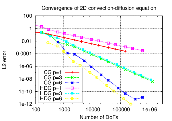 | 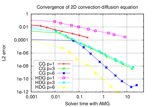 |
The results in the graphs show that the HDG method is slower than continuous finite elements at \(p=1\), about equally fast for cubic elements and faster for sixth order elements. However, we have seen above that the HDG method actually produces solutions which are more accurate than what is represented in the original variables. Therefore, in the next two plots below we instead display the error of the post-processed solution for HDG (denoted by \(p=1^*\) for example). We now see a clear advantage of HDG for the same amount of work for both \(p=3\) and \(p=6\), and about the same quality for \(p=1\).
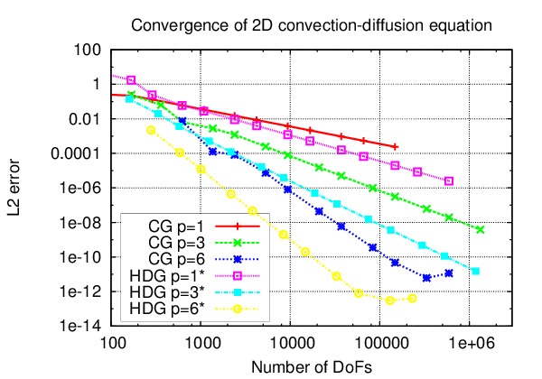 | 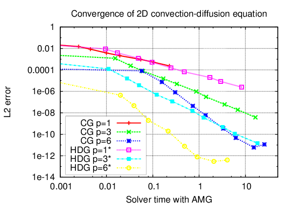 |
Since the HDG method actually produces results converging as \(h^{p+2}\), we should compare it to a continuous Galerkin solution with the same asymptotic convergence behavior, i.e., FE_Q with degree \(p+1\). If we do this, we get the convergence curves below. We see that CG with second order polynomials is again clearly better than HDG with linears. However, the advantage of HDG for higher orders remains.
The results are in line with properties of DG methods in general: Best performance is typically not achieved for linear elements, but rather at somewhat higher order, usually around \(p=3\). This is because of a volume-to-surface effect for discontinuous solutions with too much of the solution living on the surfaces and hence duplicating work when the elements are linear. Put in other words, DG methods are often most efficient when used at relatively high order, despite their focus on a discontinuous (and hence, seemingly low accurate) representation of solutions.
Results for 3D
We now show the same figures in 3D: The first row shows the number of degrees of freedom and computing time versus the \(L_2\) error in the scalar variable \(u\) for CG and HDG at order \(p\), the second row shows the post-processed HDG solution instead of the original one, and the third row compares the post-processed HDG solution with CG at order \(p+1\). In 3D, the volume-to-surface effect makes the cost of HDG somewhat higher and the CG solution is clearly better than HDG for linears by any metric. For cubics, HDG and CG are of similar quality, whereas HDG is again more efficient for sixth order polynomials. One can alternatively also use the combination of FE_DGP and FE_FaceP instead of (FE_DGQ, FE_FaceQ), which do not use tensor product polynomials of degree \(p\) but Legendre polynomials of complete degree \(p\). There are fewer degrees of freedom on the skeleton variable for FE_FaceP for a given mesh size, but the solution quality (error vs. number of DoFs) is very similar to the results for FE_FaceQ.
One final note on the efficiency comparison: We tried to use general-purpose sparse matrix structures and similar solvers (optimal AMG preconditioners for both without particular tuning of the AMG parameters on any of them) to give a fair picture of the cost versus accuracy of two methods, on a toy example. It should be noted however that geometric multigrid (GMG) for continuous finite elements is about a factor four to five faster for \(p=3\) and \(p=6\). As of 2019, optimal-complexity iterative solvers for HDG are still under development in the research community. Also, there are other implementation aspects for CG available such as fast matrix-free approaches as shown in step-37 that make higher order continuous elements more competitive. Again, it is not clear to the authors of the tutorial whether similar improvements could be made for HDG. We refer to Kronbichler and Wall (2018) for a recent efficiency evaluation.
Possibilities for improvements
As already mentioned in the introduction, one possibility is to implement another post-processing technique as discussed in the literature.
A second item that is not done optimally relates to the performance of this program, which is of course an issue in practical applications (weighing in also the better solution quality of (H)DG methods for transport-dominated problems). Let us look at the computing time of the tutorial program and the share of the individual components:
| | | Setup | Assemble | Solve | Trace reconstruct | Post-processing | Output |
| | Total time | Relative share |
| 2D, Q1, cycle 9, 37,248 dofs | 5.34s | 0.7% | 1.2% | 89.5% | 0.9% | 2.3% | 5.4% |
| 2D, Q3, cycle 9, 74,496 dofs | 22.2s | 0.4% | 4.3% | 84.1% | 4.1% | 3.5% | 3.6% |
| 3D, Q1, cycle 7, 172,800 dofs | 9.06s | 3.1% | 8.9% | 42.7% | 7.0% | 20.6% | 17.7% |
| 3D, Q3, cycle 7, 691,200 dofs | 516s | 0.6% | 34.5% | 13.4% | 32.8% | 17.1% | 1.5% |
As can be seen from the table, the solver and assembly calls dominate the runtime of the program. This also gives a clear indication of where improvements would make the most sense:
-
Better linear solvers: We use a BiCGStab iterative solver without preconditioner, where the number of iteration increases with increasing problem size (the number of iterations for Q1 elements and global refinements starts at 35 for the small sizes but increase up to 701 for the largest size). To do better, one could for example use an algebraic multigrid preconditioner from Trilinos, or some more advanced variants as the one discussed in Kronbichler and Wall (2018). For diffusion-dominated problems such as the problem at hand with finer meshes, such a solver can be designed that uses the matrix-vector products from the more efficient ChunkSparseMatrix on the finest level, as long as we are not working in parallel with MPI. For MPI-parallelized computations, a standard TrilinosWrappers::SparseMatrix can be used.
-
Speed up assembly by pre-assembling parts that do not change from one cell to another (those that do neither contain variable coefficients nor mapping-dependent terms).
The plain program
#include <iostream>
namespace Step51
{
template <int dim>
class SolutionBase
{
protected:
static const unsigned int n_source_centers = 3;
static const Point<dim> source_centers[n_source_centers];
static const double width;
};
template <>
SolutionBase<1>::source_centers[SolutionBase<1>::n_source_centers] =
template <>
SolutionBase<2>::source_centers[SolutionBase<2>::n_source_centers] =
template <>
SolutionBase<3>::source_centers[SolutionBase<3>::n_source_centers] = {
template <int dim>
const double SolutionBase<dim>::width = 1. / 5.;
template <int dim>
class Solution :
public Function<dim>,
protected SolutionBase<dim>
{
public:
const unsigned int = 0) const override
{
for (unsigned int i = 0; i < this->n_source_centers; ++i)
{
}
}
const unsigned int = 0) const override
{
for (unsigned int i = 0; i < this->n_source_centers; ++i)
{
(-2 / (this->width * this->width) *
std::exp(-x_minus_xi.
norm_square() / (this->width * this->width)) *
x_minus_xi);
}
}
};
template <int dim>
class SolutionAndGradient :
public Function<dim>,
protected SolutionBase<dim>
{
public:
SolutionAndGradient()
{}
{
Solution<dim> solution;
for (
unsigned int d = 0;
d < dim; ++
d)
v[dim] = solution.value(p);
}
};
template <int dim>
{
public:
ConvectionVelocity()
{}
{
switch (dim)
{
case 1:
convection[0] = 1;
break;
case 2:
convection[0] = p[1];
convection[1] = -p[0];
break;
case 3:
convection[0] = p[1];
convection[1] = -p[0];
convection[2] = 1;
break;
default:
}
return convection;
}
};
template <int dim>
class RightHandSide :
public Function<dim>,
protected SolutionBase<dim>
{
public:
const unsigned int = 0) const override
{
ConvectionVelocity<dim> convection_velocity;
for (unsigned int i = 0; i < this->n_source_centers; ++i)
{
((2 * dim - 2 * convection * x_minus_xi -
4 * x_minus_xi.
norm_square() / (this->width * this->width)) /
(this->width * this->width) *
std::exp(-x_minus_xi.
norm_square() / (this->width * this->width)));
}
}
};
template <int dim>
class HDG
{
public:
enum RefinementMode
{
global_refinement,
adaptive_refinement
};
HDG(const unsigned int degree, const RefinementMode refinement_mode);
private:
void setup_system();
void assemble_system(const bool reconstruct_trace = false);
void solve();
void postprocess();
void refine_grid(const unsigned int cycle);
void output_results(const unsigned int cycle);
struct PerTaskData;
struct ScratchData;
struct PostProcessScratchData;
void assemble_system_one_cell(
ScratchData & scratch,
PerTaskData & task_data);
void copy_local_to_global(const PerTaskData &data);
void postprocess_one_cell(
PostProcessScratchData & scratch,
unsigned int & empty_data);
const RefinementMode refinement_mode;
};
template <int dim>
HDG<dim>::HDG(const unsigned int degree, const RefinementMode refinement_mode)
: fe_local(
FE_DGQ<dim>(degree), dim,
FE_DGQ<dim>(degree), 1)
, fe(degree)
, fe_u_post(degree + 1)
, refinement_mode(refinement_mode)
{}
template <int dim>
void HDG<dim>::setup_system()
{
dof_handler_u_post.distribute_dofs(fe_u_post);
std::cout <<
" Number of degrees of freedom: " << dof_handler.
n_dofs()
<< std::endl;
solution.reinit(dof_handler.
n_dofs());
solution_local.reinit(dof_handler_local.n_dofs());
solution_u_post.reinit(dof_handler_u_post.n_dofs());
constraints.clear();
std::map<types::boundary_id, const Function<dim> *> boundary_functions;
Solution<dim> solution_function;
boundary_functions[0] = &solution_function;
boundary_functions,
constraints);
constraints.close();
{
}
system_matrix.reinit(sparsity_pattern);
}
template <int dim>
struct HDG<dim>::PerTaskData
{
std::vector<types::global_dof_index> dof_indices;
bool trace_reconstruct;
PerTaskData(const unsigned int n_dofs, const bool trace_reconstruct)
, cell_vector(n_dofs)
, dof_indices(n_dofs)
, trace_reconstruct(trace_reconstruct)
{}
};
template <int dim>
struct HDG<dim>::ScratchData
{
std::vector<Tensor<1, dim>> q_phi;
std::vector<double> q_phi_div;
std::vector<double> u_phi;
std::vector<Tensor<1, dim>> u_phi_grad;
std::vector<double> tr_phi;
std::vector<double> trace_values;
std::vector<std::vector<unsigned int>> fe_local_support_on_face;
std::vector<std::vector<unsigned int>> fe_support_on_face;
ConvectionVelocity<dim> convection_velocity;
RightHandSide<dim> right_hand_side;
const Solution<dim> exact_solution;
: fe_values_local(fe_local, quadrature_formula, local_flags)
, fe_face_values_local(fe_local,
face_quadrature_formula,
local_face_flags)
, fe_face_values(fe, face_quadrature_formula, flags)
, ll_matrix(fe_local.dofs_per_cell, fe_local.dofs_per_cell)
, lf_matrix(fe_local.dofs_per_cell, fe.dofs_per_cell)
, fl_matrix(fe.dofs_per_cell, fe_local.dofs_per_cell)
, tmp_matrix(fe.dofs_per_cell, fe_local.dofs_per_cell)
, l_rhs(fe_local.dofs_per_cell)
, tmp_rhs(fe_local.dofs_per_cell)
, q_phi(fe_local.dofs_per_cell)
, q_phi_div(fe_local.dofs_per_cell)
, u_phi(fe_local.dofs_per_cell)
, u_phi_grad(fe_local.dofs_per_cell)
, tr_phi(fe.dofs_per_cell)
, trace_values(face_quadrature_formula.size())
, fe_local_support_on_face(
GeometryInfo<dim>::faces_per_cell)
, exact_solution()
{
{
fe_local_support_on_face[face_no].push_back(i);
}
{
fe_support_on_face[face_no].push_back(i);
}
}
ScratchData(const ScratchData &sd)
: fe_values_local(sd.fe_values_local.get_fe(),
sd.fe_values_local.get_quadrature(),
sd.fe_values_local.get_update_flags())
, fe_face_values_local(sd.fe_face_values_local.get_fe(),
sd.fe_face_values_local.get_quadrature(),
sd.fe_face_values_local.get_update_flags())
, fe_face_values(sd.fe_face_values.get_fe(),
sd.fe_face_values.get_quadrature(),
sd.fe_face_values.get_update_flags())
, ll_matrix(sd.ll_matrix)
, lf_matrix(sd.lf_matrix)
, fl_matrix(sd.fl_matrix)
, tmp_matrix(sd.tmp_matrix)
, l_rhs(sd.l_rhs)
, tmp_rhs(sd.tmp_rhs)
, q_phi(sd.q_phi)
, q_phi_div(sd.q_phi_div)
, u_phi(sd.u_phi)
, u_phi_grad(sd.u_phi_grad)
, tr_phi(sd.tr_phi)
, trace_values(sd.trace_values)
, fe_local_support_on_face(sd.fe_local_support_on_face)
, fe_support_on_face(sd.fe_support_on_face)
, exact_solution()
{}
};
template <int dim>
struct HDG<dim>::PostProcessScratchData
{
std::vector<double> u_values;
std::vector<Tensor<1, dim>> u_gradients;
: fe_values_local(fe_local, quadrature_formula, local_flags)
, fe_values(fe, quadrature_formula, flags)
, u_values(quadrature_formula.size())
, u_gradients(quadrature_formula.size())
, cell_rhs(fe.dofs_per_cell)
, cell_sol(fe.dofs_per_cell)
{}
PostProcessScratchData(const PostProcessScratchData &sd)
: fe_values_local(sd.fe_values_local.get_fe(),
sd.fe_values_local.get_quadrature(),
sd.fe_values_local.get_update_flags())
, fe_values(sd.fe_values.get_fe(),
sd.fe_values.get_quadrature(),
sd.fe_values.get_update_flags())
, u_values(sd.u_values)
, u_gradients(sd.u_gradients)
, cell_rhs(sd.cell_rhs)
, cell_sol(sd.cell_sol)
{}
};
template <int dim>
void HDG<dim>::assemble_system(const bool trace_reconstruct)
{
const QGauss<dim - 1> face_quadrature_formula(fe.
degree + 1);
ScratchData scratch(fe,
fe_local,
quadrature_formula,
face_quadrature_formula,
local_flags,
local_face_flags,
flags);
*this,
&HDG<dim>::assemble_system_one_cell,
&HDG<dim>::copy_local_to_global,
scratch,
task_data);
}
template <int dim>
void HDG<dim>::assemble_system_one_cell(
ScratchData & scratch,
PerTaskData & task_data)
{
cell->level(),
cell->index(),
&dof_handler_local);
const unsigned int n_q_points =
scratch.fe_values_local.get_quadrature().size();
const unsigned int n_face_q_points =
scratch.fe_face_values_local.get_quadrature().size();
const unsigned int loc_dofs_per_cell =
scratch.fe_values_local.get_fe().dofs_per_cell;
scratch.ll_matrix = 0;
scratch.l_rhs = 0;
if (!task_data.trace_reconstruct)
{
scratch.lf_matrix = 0;
scratch.fl_matrix = 0;
task_data.cell_matrix = 0;
task_data.cell_vector = 0;
}
scratch.fe_values_local.reinit(loc_cell);
for (unsigned int q = 0; q < n_q_points; ++q)
{
const double rhs_value = scratch.right_hand_side.value(
scratch.fe_values_local.quadrature_point(q));
scratch.fe_values_local.quadrature_point(q));
const double JxW = scratch.fe_values_local.JxW(q);
for (unsigned int k = 0; k < loc_dofs_per_cell; ++k)
{
scratch.q_phi[k] = scratch.fe_values_local[fluxes].value(k, q);
scratch.q_phi_div[k] =
scratch.fe_values_local[fluxes].divergence(k, q);
scratch.u_phi[k] = scratch.fe_values_local[scalar].value(k, q);
scratch.u_phi_grad[k] =
scratch.fe_values_local[scalar].gradient(k, q);
}
for (unsigned int i = 0; i < loc_dofs_per_cell; ++i)
{
for (unsigned int j = 0; j < loc_dofs_per_cell; ++j)
scratch.ll_matrix(i, j) +=
(scratch.q_phi[i] * scratch.q_phi[j] -
scratch.q_phi_div[i] * scratch.u_phi[j] +
scratch.u_phi[i] * scratch.q_phi_div[j] -
(scratch.u_phi_grad[i] * convection) * scratch.u_phi[j]) *
JxW;
scratch.l_rhs(i) += scratch.u_phi[i] * rhs_value * JxW;
}
}
{
scratch.fe_face_values_local.reinit(loc_cell, face_no);
scratch.fe_face_values.reinit(cell, face_no);
if (task_data.trace_reconstruct)
scratch.fe_face_values.get_function_values(solution,
scratch.trace_values);
for (unsigned int q = 0; q < n_face_q_points; ++q)
{
const double JxW = scratch.fe_face_values.JxW(q);
scratch.fe_face_values.quadrature_point(q);
scratch.fe_face_values.normal_vector(q);
scratch.convection_velocity.value(quadrature_point);
const double tau_stab = (5. +
std::abs(convection * normal));
for (unsigned int k = 0;
k < scratch.fe_local_support_on_face[face_no].size();
++k)
{
const unsigned int kk =
scratch.fe_local_support_on_face[face_no][k];
scratch.q_phi[k] =
scratch.fe_face_values_local[fluxes].value(kk, q);
scratch.u_phi[k] =
scratch.fe_face_values_local[scalar].value(kk, q);
}
if (!task_data.trace_reconstruct)
{
for (unsigned int k = 0;
k < scratch.fe_support_on_face[face_no].size();
++k)
scratch.tr_phi[k] = scratch.fe_face_values.shape_value(
scratch.fe_support_on_face[face_no][k], q);
for (unsigned int i = 0;
i < scratch.fe_local_support_on_face[face_no].size();
++i)
for (unsigned int j = 0;
j < scratch.fe_support_on_face[face_no].size();
++j)
{
const unsigned int ii =
scratch.fe_local_support_on_face[face_no][i];
const unsigned int jj =
scratch.fe_support_on_face[face_no][j];
scratch.lf_matrix(ii, jj) +=
((scratch.q_phi[i] * normal +
(convection * normal - tau_stab) * scratch.u_phi[i]) *
scratch.tr_phi[j]) *
JxW;
scratch.fl_matrix(jj, ii) -=
((scratch.q_phi[i] * normal +
tau_stab * scratch.u_phi[i]) *
scratch.tr_phi[j]) *
JxW;
}
for (unsigned int i = 0;
i < scratch.fe_support_on_face[face_no].size();
++i)
for (unsigned int j = 0;
j < scratch.fe_support_on_face[face_no].size();
++j)
{
const unsigned int ii =
scratch.fe_support_on_face[face_no][i];
const unsigned int jj =
scratch.fe_support_on_face[face_no][j];
task_data.cell_matrix(ii, jj) +=
((convection * normal - tau_stab) * scratch.tr_phi[i] *
scratch.tr_phi[j]) *
JxW;
}
if (cell->face(face_no)->at_boundary() &&
(cell->face(face_no)->boundary_id() == 1))
{
const double neumann_value =
-scratch.exact_solution.gradient(quadrature_point) *
normal +
convection * normal *
scratch.exact_solution.value(quadrature_point);
for (unsigned int i = 0;
i < scratch.fe_support_on_face[face_no].size();
++i)
{
const unsigned int ii =
scratch.fe_support_on_face[face_no][i];
task_data.cell_vector(ii) +=
scratch.tr_phi[i] * neumann_value * JxW;
}
}
}
for (unsigned int i = 0;
i < scratch.fe_local_support_on_face[face_no].size();
++i)
for (unsigned int j = 0;
j < scratch.fe_local_support_on_face[face_no].size();
++j)
{
const unsigned int ii =
scratch.fe_local_support_on_face[face_no][i];
const unsigned int jj =
scratch.fe_local_support_on_face[face_no][j];
scratch.ll_matrix(ii, jj) +=
tau_stab * scratch.u_phi[i] * scratch.u_phi[j] * JxW;
}
if (task_data.trace_reconstruct)
for (unsigned int i = 0;
i < scratch.fe_local_support_on_face[face_no].size();
++i)
{
const unsigned int ii =
scratch.fe_local_support_on_face[face_no][i];
scratch.l_rhs(ii) -=
(scratch.q_phi[i] * normal +
scratch.u_phi[i] * (convection * normal - tau_stab)) *
scratch.trace_values[q] * JxW;
}
}
}
scratch.ll_matrix.gauss_jordan();
if (task_data.trace_reconstruct == false)
{
scratch.fl_matrix.mmult(scratch.tmp_matrix, scratch.ll_matrix);
scratch.tmp_matrix.vmult_add(task_data.cell_vector, scratch.l_rhs);
scratch.tmp_matrix.mmult(task_data.cell_matrix,
scratch.lf_matrix,
true);
cell->get_dof_indices(task_data.dof_indices);
}
else
{
scratch.ll_matrix.vmult(scratch.tmp_rhs, scratch.l_rhs);
loc_cell->set_dof_values(scratch.tmp_rhs, solution_local);
}
}
template <int dim>
void HDG<dim>::copy_local_to_global(const PerTaskData &data)
{
if (data.trace_reconstruct == false)
constraints.distribute_local_to_global(data.cell_matrix,
data.cell_vector,
data.dof_indices,
system_matrix,
system_rhs);
}
template <int dim>
void HDG<dim>::solve()
{
std::cout << " Number of BiCGStab iterations: "
<< solver_control.last_step() << std::endl;
system_matrix.clear();
sparsity_pattern.
reinit(0, 0, 0, 1);
constraints.distribute(solution);
assemble_system(true);
}
template <int dim>
void HDG<dim>::postprocess()
{
{
const QGauss<dim> quadrature_formula(fe_u_post.degree + 1);
PostProcessScratchData scratch(
fe_u_post, fe_local, quadrature_formula, local_flags, flags);
dof_handler_u_post.begin_active(),
dof_handler_u_post.end(),
PostProcessScratchData & scratch,
unsigned int & data) {
this->postprocess_one_cell(cell, scratch, data);
},
std::function<void(const unsigned int &)>(),
scratch,
}
Vector<float> difference_per_cell(
triangulation.n_active_cells());
solution_local,
SolutionAndGradient<dim>(),
difference_per_cell,
&value_select);
const double L2_error =
difference_per_cell,
std::pair<unsigned int, unsigned int>(0, dim), dim + 1);
solution_local,
SolutionAndGradient<dim>(),
difference_per_cell,
&gradient_select);
const double grad_error =
difference_per_cell,
solution_u_post,
Solution<dim>(),
difference_per_cell,
const double post_error =
difference_per_cell,
convergence_table.add_value(
"cells",
triangulation.n_active_cells());
convergence_table.add_value(
"dofs", dof_handler.
n_dofs());
convergence_table.add_value("val L2", L2_error);
convergence_table.set_scientific("val L2", true);
convergence_table.set_precision("val L2", 3);
convergence_table.add_value("grad L2", grad_error);
convergence_table.set_scientific("grad L2", true);
convergence_table.set_precision("grad L2", 3);
convergence_table.add_value("val L2-post", post_error);
convergence_table.set_scientific("val L2-post", true);
convergence_table.set_precision("val L2-post", 3);
}
template <int dim>
void HDG<dim>::postprocess_one_cell(
PostProcessScratchData & scratch,
unsigned int &)
{
cell->level(),
cell->index(),
&dof_handler_local);
scratch.fe_values_local.reinit(loc_cell);
scratch.fe_values.reinit(cell);
const unsigned int n_q_points = scratch.fe_values.get_quadrature().size();
const unsigned int dofs_per_cell = scratch.fe_values.dofs_per_cell;
scratch.fe_values_local[scalar].get_function_values(solution_local,
scratch.u_values);
scratch.fe_values_local[fluxes].get_function_values(solution_local,
scratch.u_gradients);
for (unsigned int i = 1; i < dofs_per_cell; ++i)
{
for (unsigned int j = 0; j < dofs_per_cell; ++j)
{
for (unsigned int q = 0; q < n_q_points; ++q)
sum += (scratch.fe_values.shape_grad(i, q) *
scratch.fe_values.shape_grad(j, q)) *
scratch.fe_values.JxW(q);
scratch.cell_matrix(i, j) =
sum;
}
for (unsigned int q = 0; q < n_q_points; ++q)
sum -= (scratch.fe_values.shape_grad(i, q) * scratch.u_gradients[q]) *
scratch.fe_values.JxW(q);
scratch.cell_rhs(i) =
sum;
}
for (unsigned int j = 0; j < dofs_per_cell; ++j)
{
for (unsigned int q = 0; q < n_q_points; ++q)
sum += scratch.fe_values.shape_value(j, q) * scratch.fe_values.JxW(q);
scratch.cell_matrix(0, j) =
sum;
}
{
for (unsigned int q = 0; q < n_q_points; ++q)
sum += scratch.u_values[q] * scratch.fe_values.JxW(q);
scratch.cell_rhs(0) =
sum;
}
scratch.cell_matrix.gauss_jordan();
scratch.cell_matrix.vmult(scratch.cell_sol, scratch.cell_rhs);
cell->distribute_local_to_global(scratch.cell_sol, solution_u_post);
}
template <int dim>
void HDG<dim>::output_results(const unsigned int cycle)
{
std::string filename;
switch (refinement_mode)
{
case global_refinement:
filename = "solution-global";
break;
case adaptive_refinement:
filename = "solution-adaptive";
break;
default:
}
std::string face_out(filename);
face_out += "-face";
filename += ".vtk";
std::ofstream output(filename);
std::vector<std::string> names(dim, "gradient");
names.emplace_back("solution");
std::vector<DataComponentInterpretation::DataComponentInterpretation>
component_interpretation(
component_interpretation[dim] =
solution_local,
names,
component_interpretation);
std::vector<std::string> post_name(1, "u_post");
std::vector<DataComponentInterpretation::DataComponentInterpretation>
solution_u_post,
post_name,
post_comp_type);
face_out += ".vtk";
std::ofstream face_output(face_out);
std::vector<std::string> face_name(1, "u_hat");
std::vector<DataComponentInterpretation::DataComponentInterpretation>
data_out_face.add_data_vector(dof_handler,
solution,
face_name,
face_component_type);
data_out_face.build_patches(fe.
degree);
data_out_face.write_vtk(face_output);
}
template <int dim>
void HDG<dim>::refine_grid(const unsigned int cycle)
{
if (cycle == 0)
{
}
else
switch (refinement_mode)
{
case global_refinement:
{
2 + (cycle % 2),
-1,
1);
break;
}
case adaptive_refinement:
{
Vector<float> estimated_error_per_cell(
std::map<types::boundary_id, const Function<dim> *>
neumann_boundary;
neumann_boundary,
solution_local,
estimated_error_per_cell,
scalar));
break;
}
default:
{
}
}
for (const auto &face : cell->face_iterators())
if (face->at_boundary())
if ((
std::fabs(face->center()(0) - (-1)) < 1
e-12) ||
face->set_boundary_id(1);
}
template <int dim>
{
for (unsigned int cycle = 0; cycle < 10; ++cycle)
{
std::cout << "Cycle " << cycle << ':' << std::endl;
refine_grid(cycle);
setup_system();
assemble_system(false);
solve();
postprocess();
output_results(cycle);
}
if (refinement_mode == global_refinement)
{
convergence_table.evaluate_convergence_rates(
convergence_table.evaluate_convergence_rates(
convergence_table.evaluate_convergence_rates(
}
convergence_table.write_text(std::cout);
}
}
int main()
{
const unsigned int dim = 2;
try
{
{
std::cout << "Solving with Q1 elements, adaptive refinement"
<< std::endl
<< "============================================="
<< std::endl
<< std::endl;
Step51::HDG<dim> hdg_problem(1, Step51::HDG<dim>::adaptive_refinement);
hdg_problem.run();
std::cout << std::endl;
}
{
std::cout << "Solving with Q1 elements, global refinement" << std::endl
<< "===========================================" << std::endl
<< std::endl;
Step51::HDG<dim> hdg_problem(1, Step51::HDG<dim>::global_refinement);
hdg_problem.run();
std::cout << std::endl;
}
{
std::cout << "Solving with Q3 elements, global refinement" << std::endl
<< "===========================================" << std::endl
<< std::endl;
Step51::HDG<dim> hdg_problem(3, Step51::HDG<dim>::global_refinement);
hdg_problem.run();
std::cout << std::endl;
}
}
catch (std::exception &exc)
{
std::cerr << std::endl
<< std::endl
<< "----------------------------------------------------"
<< std::endl;
std::cerr << "Exception on processing: " << std::endl
<< exc.what() << std::endl
<< "Aborting!" << std::endl
<< "----------------------------------------------------"
<< std::endl;
return 1;
}
catch (...)
{
std::cerr << std::endl
<< std::endl
<< "----------------------------------------------------"
<< std::endl;
std::cerr << "Unknown exception!" << std::endl
<< "Aborting!" << std::endl
<< "----------------------------------------------------"
<< std::endl;
return 1;
}
return 0;
}


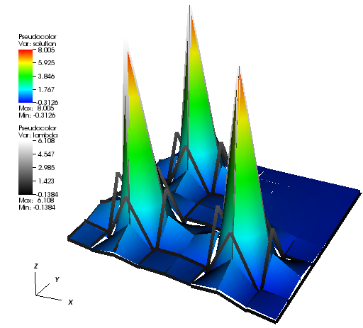
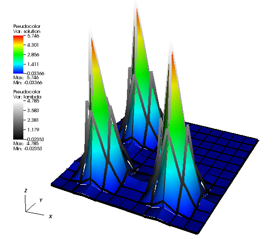
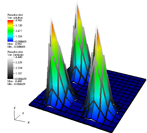


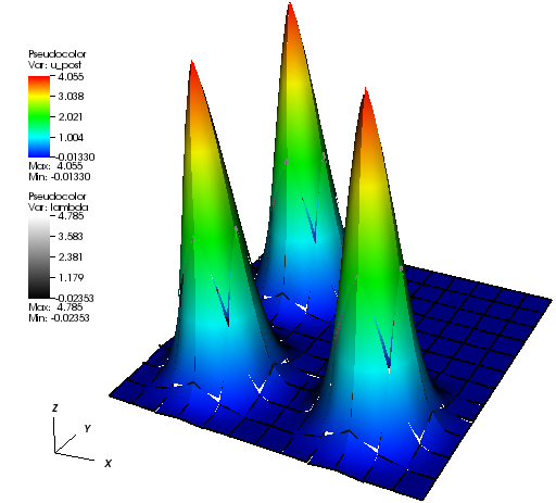

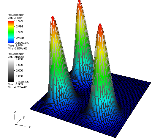
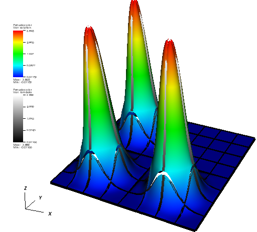
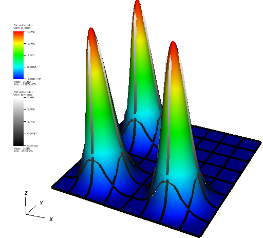


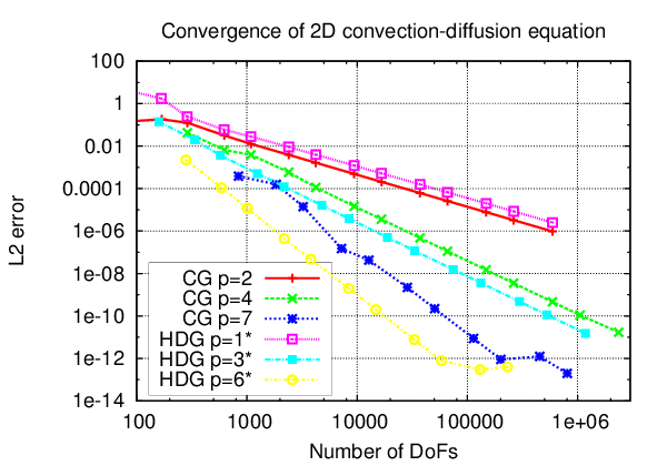
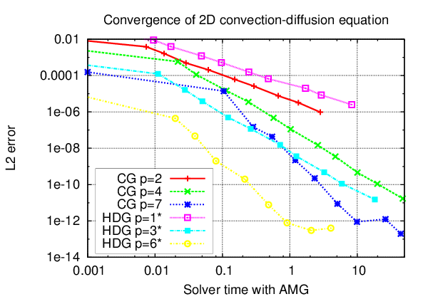
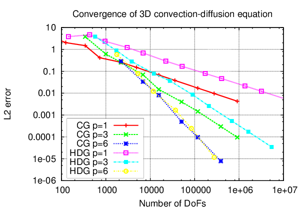
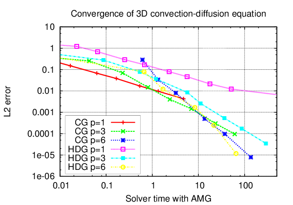
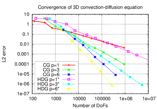
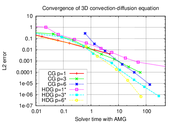
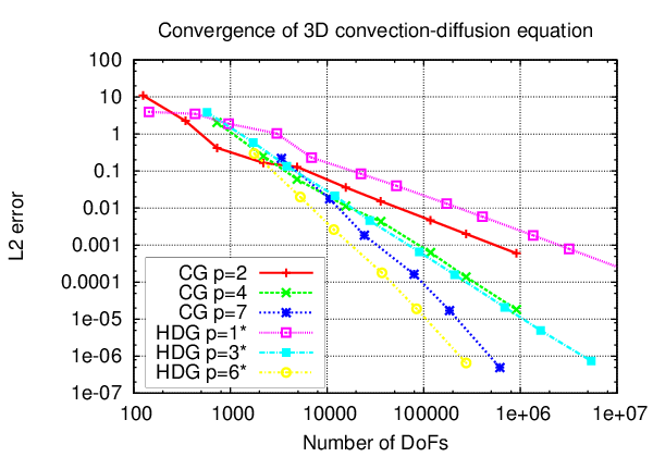
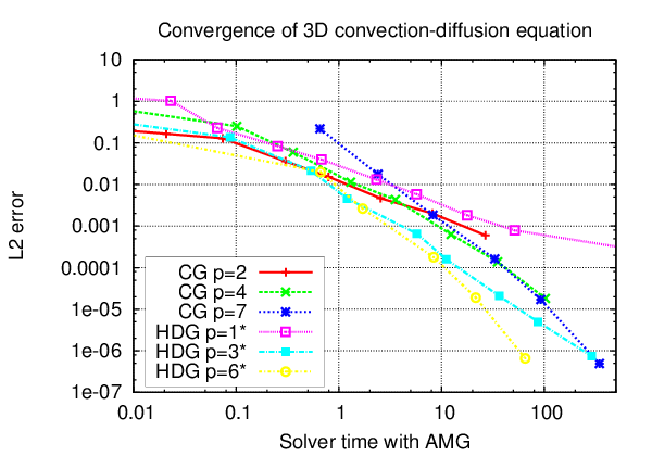
 1.8.17