 |
Reference documentation for deal.II version 9.2.0
|
 |
Reference documentation for deal.II version 9.2.0
|
This tutorial depends on step-6.
| Table of contents | |
|---|---|
In this example program, we will not so much be concerned with describing new ways how to use deal.II and its facilities, but rather with presenting methods of writing modular and extensible finite element programs. The main reason for this is the size and complexity of modern research software: applications implementing modern error estimation concepts and adaptive solution methods tend to become rather large. For example, when this program was written in 2002, the three largest applications by the main authors of deal.II, are at the time of writing of this example program:
(The library proper - without example programs and test suite - has slightly more than 150,000 lines of code as of spring 2002. It is of course several times larger now.) The sizes of these applications are at the edge of what one person, even an experienced programmer, can manage.
The numbers above make one thing rather clear: monolithic programs that are not broken up into smaller, mostly independent pieces have no way of surviving, since even the author will quickly lose the overview of the various dependencies between different parts of a program. Only data encapsulation, for example using object oriented programming methods, and modularization by defining small but fixed interfaces can help structure data flow and mutual interdependencies. It is also an absolute prerequisite if more than one person is developing a program, since otherwise confusion will quickly prevail as one developer would need to know if another changed something about the internals of a different module if they were not cleanly separated.
In previous examples, you have seen how the library itself is broken up into several complexes each building atop the underlying ones, but relatively independent of the other ones:
Besides these, and a large number of smaller classes, there are of course the following "tool" modules:
These complexes can also be found as a flow chart on the front page of the deal.II manual website.
The goal of this program is now to give an example of how a relatively simple finite element program could be structured such that we end up with a set of modules that are as independent of each other as possible. This allows to change the program at one end, without having to worry that it might break at the other, as long as we do not touch the interface through which the two ends communicate. The interface in C++, of course, is the declaration of abstract base classes.
Here, we will implement (again) a Laplace solver, although with a number of differences compared to previous example programs:
The things the program does are not new. In fact, this is more like a melange of previous programs, cannibalizing various parts and functions from earlier examples. It is the way they are arranged in this program that should be the focus of the reader, i.e. the software design techniques used in the program to achieve the goal of implementing the desired mathematical method. However, we must stress that software design is in part also a subjective matter: different persons have different programming backgrounds and have different opinions about the "right" style of programming; this program therefore expresses only what the author considers useful practice, and is not necessarily a style that you have to adopt in order to write successful numerical software if you feel uncomfortable with the chosen ways. It should serve as a case study, however, inspiring the reader with ideas to the desired end.
Once you have worked through the program, you will remark that it is already somewhat complex in its structure. Nevertheless, it only has about 850 lines of code, without comments. In real applications, there would of course be comments and class documentation, which would bring that to maybe 1200 lines. Yet, compared to the applications listed above, this is still small, as they are 20 to 25 times as large. For programs as large, a proper design right from the start is thus indispensable. Otherwise, it will have to be redesigned at one point in its life, once it becomes too large to be manageable.
Despite of this, all three programs listed above have undergone major revisions, or even rewrites. The wave program, for example, was once entirely teared to parts when it was still significantly smaller, just to assemble it again in a more modular form. By that time, it had become impossible to add functionality without affecting older parts of the code (the main problem with the code was the data flow: in time dependent application, the major concern is when to store data to disk and when to reload it again; if this is not done in an organized fashion, then you end up with data released too early, loaded too late, or not released at all). Although the present example program thus draws from several years of experience, it is certainly not without flaws in its design, and in particular might not be suited for an application where the objective is different. It should serve as an inspiration for writing your own application in a modular way, to avoid the pitfalls of too closely coupled codes.
What the program actually does is not even the main point of this program, the structure of the program is more important. However, in a few words, a description would be: solve the Laplace equation for a given right hand side such that the solution is the function u(x,t)=\exp(x+\sin(10y+5x^2)). The goal of the computation is to get the value of the solution at the point x_0=(0.5,0.5), and to compare the accuracy with which we resolve this value for two refinement criteria, namely global refinement and refinement by the error indicator by Kelly et al. which we have already used in previous examples.
The results will, as usual, be discussed in the respective section of this document. In doing so, we will find a slightly irritating observation about the relative performance of the two refinement criteria. In a later example program, building atop this one, we will devise a different method that should hopefully perform better than the techniques discussed here.
So much now for all the theoretical and anecdotal background. The best way of learning about a program is to look at it, so here it is:
As in all programs, we start with a list of include files from the library, and as usual they are in the standard order which is base – lac – grid – dofs – fe – numerics (as each of these categories roughly builds upon previous ones), then C++ standard headers:
Now for the C++ standard headers:
The last step is as in all previous programs:
As for the program itself, we first define classes that evaluate the solutions of a Laplace equation. In fact, they can evaluate every kind of solution, as long as it is described by a DoFHandler object, and a solution vector. We define them here first, even before the classes that actually generate the solution to be evaluated, since we need to declare an abstract base class that the solver classes can refer to.
From an abstract point of view, we declare a pure base class that provides an evaluation operator() which will do the evaluation of the solution (whatever derived classes might consider an evaluation). Since this is the only real function of this base class (except for some bookkeeping machinery), one usually terms such a class that only has an operator() a functor in C++ terminology, since it is used just like a function object.
Objects of this functor type will then later be passed to the solver object, which applies it to the solution just computed. The evaluation objects may then extract any quantity they like from the solution. The advantage of putting these evaluation functions into a separate hierarchy of classes is that by design they cannot use the internals of the solver object and are therefore independent of changes to the way the solver works. Furthermore, it is trivial to write another evaluation class without modifying the solver class, which speeds up programming (not being able to use internals of another class also means that you do not have to worry about them – programming evaluators is usually a rather quickly done task), as well as compilation (if solver and evaluation classes are put into different files: the solver only needs to see the declaration of the abstract base class, and therefore does not need to be recompiled upon addition of a new evaluation class, or modification of an old one). On a related note, you can reuse the evaluation classes for other projects, solving different equations.
In order to improve separation of code into different modules, we put the evaluation classes into a namespace of their own. This makes it easier to actually solve different equations in the same program, by assembling it from existing building blocks. The reason for this is that classes for similar purposes tend to have the same name, although they were developed in different contexts. In order to be able to use them together in one program, it is necessary that they are placed in different namespaces. This we do here:
Now for the abstract base class of evaluation classes: its main purpose is to declare a pure virtual function operator() taking a DoFHandler object, and the solution vector. In order to be able to use pointers to this base class only, it also has to declare a virtual destructor, which however does nothing. Besides this, it only provides for a little bit of bookkeeping: since we usually want to evaluate solutions on subsequent refinement levels, we store the number of the present refinement cycle, and provide a function to change this number.
The next thing is to implement actual evaluation classes. As noted in the introduction, we'd like to extract a point value from the solution, so the first class does this in its operator(). The actual point is given to this class through the constructor, as well as a table object into which it will put its findings.
Finding out the value of a finite element field at an arbitrary point is rather difficult, if we cannot rely on knowing the actual finite element used, since then we cannot, for example, interpolate between nodes. For simplicity, we therefore assume here that the point at which we want to evaluate the field is actually a node. If, in the process of evaluating the solution, we find that we did not encounter this point upon looping over all vertices, we then have to throw an exception in order to signal to the calling functions that something has gone wrong, rather than silently ignore this error.
In the step-9 example program, we have already seen how such an exception class can be declared, using the DeclExceptionN macros. We use this mechanism here again.
From this, the actual declaration of this class should be evident. Note that of course even if we do not list a destructor explicitly, an implicit destructor is generated from the compiler, and it is virtual just as the one of the base class.
As for the definition, the constructor is trivial, just taking data and storing it in object-local ones:
Now for the function that is mainly of interest in this class, the computation of the point value:
First allocate a variable that will hold the point value. Initialize it with a value that is clearly bogus, so that if we fail to set it to a reasonable value, we will note at once. This may not be necessary in a function as small as this one, since we can easily see all possible paths of execution here, but it proved to be helpful for more complex cases, and so we employ this strategy here as well.
Then loop over all cells and all their vertices, and check whether a vertex matches the evaluation point. If this is the case, then extract the point value, set a flag that we have found the point of interest, and exit the loop.
In order to extract the point value from the global solution vector, pick that component that belongs to the vertex of interest, and, in case the solution is vector-valued, take the first component of it:
Note that by this we have made an assumption that is not valid always and should be documented in the class declaration if this were code for a real application rather than a tutorial program: we assume that the finite element used for the solution we try to evaluate actually has degrees of freedom associated with vertices. This, for example, does not hold for discontinuous elements, were the support points for the shape functions happen to be located at the vertices, but are not associated with the vertices but rather with the cell interior, since association with vertices would imply continuity there. It would also not hold for edge oriented elements, and the like.
Ideally, we would check this at the beginning of the function, for example by a statement like Assert (dof_handler.get_fe().dofs_per_vertex > 0, ExcNotImplemented()), which should make it quite clear what is going wrong when the exception is triggered. In this case, we omit it (which is indeed bad style), but knowing that that does not hurt here, since the statement cell->vertex_dof_index(vertex,0) would fail if we asked it to give us the DoF index of a vertex if there were none.
We stress again that this restriction on the allowed finite elements should be stated in the class documentation.
Since we found the right point, we now set the respective flag and exit the innermost loop. The outer loop will also be terminated due to the set flag.
Finally, we'd like to make sure that we have indeed found the evaluation point, since if that were not so we could not give a reasonable value of the solution there and the rest of the computations were useless anyway. So make sure through the AssertThrow macro already used in the step-9 program that we have indeed found this point. If this is not so, the macro throws an exception of the type that is given to it as second argument, but compared to a straightforward throw statement, it fills the exception object with a set of additional information, for example the source file and line number where the exception was generated, and the condition that failed. If you have a catch clause in your main function (as this program has), you will catch all exceptions that are not caught somewhere in between and thus already handled, and this additional information will help you find out what happened and where it went wrong.
Note that we have used the Assert macro in other example programs as well. It differed from the AssertThrow macro used here in that it simply aborts the program, rather than throwing an exception, and that it did so only in debug mode. It was the right macro to use to check about the size of vectors passed as arguments to functions, and the like.
However, here the situation is different: whether we find the evaluation point or not may change from refinement to refinement (for example, if the four cells around point are coarsened away, then the point may vanish after refinement and coarsening). This is something that cannot be predicted from a few number of runs of the program in debug mode, but should be checked always, also in production runs. Thus the use of the AssertThrow macro here.
Now, if we are sure that we have found the evaluation point, we can add the results into the table of results:
A different, maybe slightly odd kind of evaluation of a solution is to output it to a file in a graphical format. Since in the evaluation functions we are given a DoFHandler object and the solution vector, we have all we need to do this, so we can do it in an evaluation class. The reason for actually doing so instead of putting it into the class that computed the solution is that this way we have more flexibility: if we choose to only output certain aspects of it, or not output it at all. In any case, we do not need to modify the solver class, we just have to modify one of the modules out of which we build this program. This form of encapsulation, as above, helps us to keep each part of the program rather simple as the interfaces are kept simple, and no access to hidden data is possible.
Since this class which generates the output is derived from the common EvaluationBase base class, its main interface is the operator() function. Furthermore, it has a constructor taking a string that will be used as the base part of the file name to which output will be sent (we will augment it by a number indicating the number of the refinement cycle – the base class has this information at hand –, and a suffix), and the constructor also takes a value that indicates which format is requested, i.e. for which graphics program we shall generate output (from this we will then also generate the suffix of the filename to which we write).
Regarding the output format, the DataOutBase namespace provides an enumeration field DataOutBase::OutputFormat which lists names for all supported output formats. At the time of writing of this program, the supported graphics formats are represented by the enum values ucd, gnuplot, povray, eps, gmv, tecplot, tecplot_binary, dx, vtk, etc, but this list will certainly grow over time. Now, within various functions of that base class, you can use values of this type to get information about these graphics formats (for example the default suffix used for files of each format), and you can call a generic write function, which then branches to the write_gnuplot, write_ucd, etc functions which we have used in previous examples already, based on the value of a second argument given to it denoting the required output format. This mechanism makes it simple to write an extensible program that can decide which output format to use at runtime, and it also makes it rather simple to write the program in a way such that it takes advantage of newly implemented output formats, without the need to change the application program.
Of these two fields, the base name and the output format descriptor, the constructor takes values and stores them for later use by the actual evaluation function.
Following the description above, the function generating the actual output is now relatively straightforward. The only particularly interesting feature over previous example programs is the use of the DataOutBase::default_suffix function, returning the usual suffix for files of a given format (e.g. ".eps" for encapsulated postscript files, ".gnuplot" for Gnuplot files), and of the generic DataOut::write() function with a second argument, which internally branches to the actual output functions for the different graphics formats, based on the value of the format descriptor passed as second argument.
Also note that we have to prefix this-> to access a member variable of the template dependent base class. The reason here, and further down in the program is the same as the one described in the step-7 example program (look for two-stage name lookup there).
In practical applications, one would add here a list of other possible evaluation classes, representing quantities that one may be interested in. For this example, that much shall be sufficient, so we close the namespace.
After defining what we want to know of the solution, we should now care how to get at it. We will pack everything we need into a namespace of its own, for much the same reasons as for the evaluations above.
Since we have discussed Laplace solvers already in considerable detail in previous examples, there is not much new stuff following. Rather, we have to a great extent cannibalized previous examples and put them, in slightly different form, into this example program. We will therefore mostly be concerned with discussing the differences to previous examples.
Basically, as already said in the introduction, the lack of new stuff in this example is deliberate, as it is more to demonstrate software design practices, rather than mathematics. The emphasis in explanations below will therefore be more on the actual implementation.
In defining a Laplace solver, we start out by declaring an abstract base class, that has no functionality itself except for taking and storing a pointer to the triangulation to be used later.
This base class is very general, and could as well be used for any other stationary problem. It provides declarations of functions that shall, in derived classes, solve a problem, postprocess the solution with a list of evaluation objects, and refine the grid, respectively. None of these functions actually does something itself in the base class.
Due to the lack of actual functionality, the programming style of declaring very abstract base classes is similar to the style used in Smalltalk or Java programs, where all classes are derived from entirely abstract classes Object, even number representations. The author admits that he does not particularly like the use of such a style in C++, as it puts style over reason. Furthermore, it promotes the use of virtual functions for everything (for example, in Java, all functions are virtual per se), which, however, has proven to be rather inefficient in many applications where functions are often only accessing data, not doing computations, and therefore quickly return; the overhead of virtual functions can then be significant. The opinion of the author is to have abstract base classes wherever at least some part of the code of actual implementations can be shared and thus separated into the base class.
Besides all these theoretical questions, we here have a good reason, which will become clearer to the reader below. Basically, we want to be able to have a family of different Laplace solvers that differ so much that no larger common subset of functionality could be found. We therefore just declare such an abstract base class, taking a pointer to a triangulation in the constructor and storing it henceforth. Since this triangulation will be used throughout all computations, we have to make sure that the triangulation is valid until it is last used. We do this by keeping a SmartPointer to this triangulation, as explained in step-7.
Note that while the pointer itself is declared constant (i.e. throughout the lifetime of this object, the pointer points to the same object), it is not declared as a pointer to a constant triangulation. In fact, by this we allow that derived classes refine or coarsen the triangulation within the refine_grid function.
Finally, we have a function n_dofs is only a tool for the driver functions to decide whether we want to go on with mesh refinement or not. It returns the number of degrees of freedom the present simulation has.
The implementation of the only two non-abstract functions is then rather boring:
Following now the main class that implements assembling the matrix of the linear system, solving it, and calling the postprocessor objects on the solution. It implements the solve_problem and postprocess functions declared in the base class. It does not, however, implement the refine_grid method, as mesh refinement will be implemented in a number of derived classes.
It also declares a new abstract virtual function, assemble_rhs, that needs to be overloaded in subclasses. The reason is that we will implement two different classes that will implement different methods to assemble the right hand side vector. This function might also be interesting in cases where the right hand side depends not simply on a continuous function, but on something else as well, for example the solution of another discretized problem, etc. The latter happens frequently in non-linear problems.
As we mentioned previously, the actual content of this class is not new, but a mixture of various techniques already used in previous examples. We will therefore not discuss them in detail, but refer the reader to these programs.
Basically, in a few words, the constructor of this class takes pointers to a triangulation, a finite element, and a function object representing the boundary values. These are either passed down to the base class's constructor, or are stored and used to generate a DoFHandler object later. Since finite elements and quadrature formula should match, it is also passed a quadrature object.
The solve_problem sets up the data structures for the actual solution, calls the functions to assemble the linear system, and solves it.
The postprocess function finally takes an evaluation object and applies it to the computed solution.
The n_dofs function finally implements the pure virtual function of the base class.
In the protected section of this class, we first have a number of member variables, of which the use should be clear from the previous examples:
Then we declare an abstract function that will be used to assemble the right hand side. As explained above, there are various cases for which this action differs strongly in what is necessary, so we defer this to derived classes:
Next, in the private section, we have a small class which represents an entire linear system, i.e. a matrix, a right hand side, and a solution vector, as well as the constraints that are applied to it, such as those due to hanging nodes. Its constructor initializes the various subobjects, and there is a function that implements a conjugate gradient method as solver.
Finally, there is a set of functions which will be used to assemble the actual system matrix. The main function of this group, assemble_linear_system() computes the matrix in parallel on multicore systems, using the following two helper functions. The mechanism for doing so is the same as in the step-9 example program and follows the WorkStream concept outlined in Parallel computing with multiple processors accessing shared memory . The main function also calls the virtual function assembling the right hand side.
Now here comes the constructor of the class. It does not do much except store pointers to the objects given, and generate DoFHandler object initialized with the given pointer to a triangulation. This causes the DoF handler to store that pointer, but does not already generate a finite element numbering (we only ask for that in the solve_problem function).
The destructor is simple, it only clears the information stored in the DoF handler object to release the memory.
The next function is the one which delegates the main work in solving the problem: it sets up the DoF handler object with the finite element given to the constructor of this object, the creates an object that denotes the linear system (i.e. the matrix, the right hand side vector, and the solution vector), calls the function to assemble it, and finally solves it:
As stated above, the postprocess function takes an evaluation object, and applies it to the computed solution. This function may be called multiply, once for each evaluation of the solution which the user required.
The n_dofs function should be self-explanatory:
The following function assembles matrix and right hand side of the linear system to be solved in each step. We will do things in parallel at a couple of levels. First, note that we need to assemble both the matrix and the right hand side. These are independent operations, and we should do this in parallel. To this end, we use the concept of "tasks" that is discussed in the Parallel computing with multiple processors accessing shared memory documentation module. In essence, what we want to say "here is something that needs to be worked on, go do it whenever a CPU core is available", then do something else, and when we need the result of the first operation wait for its completion. At the second level, we want to assemble the matrix using the exact same strategy we have already used in step-9, namely the WorkStream concept.
While we could consider either assembling the right hand side or assembling the matrix as the thing to do in the background while doing the other, we will opt for the former approach simply because the call to Solver::assemble_rhs is so much simpler to write than the call to WorkStream::run with its many arguments. In any case, the code then looks like this to assemble the entire linear system:
The syntax above requires some explanation. There are multiple version of WorkStream::run that expect different arguments. In step-9, we used one version that took a pair of iterators, a pair of pointers to member functions with very specific argument lists, a pointer or reference to the object on which these member functions have to work, and a scratch and copy data object. This is a bit restrictive since the member functions called this way have to have an argument list that exactly matches what WorkStream::run expects: the local assembly function needs to take an iterator, a scratch object and a copy object; and the copy-local-to-global function needs to take exactly a copy object. But, what if we want something that's slightly more general? For example, in the current program, the copy-local-to-global function needs to know which linear system object to write the local contributions into, i.e., it also has to take a LinearSystem argument. That won't work with the approach using member function pointers.
Fortunately, C++ offers a way out. These are called function objects. In essence, what WorkStream::run wants to do is not call a member function. It wants to call some function that takes an iterator, a scratch object and a copy object in the first case, and a copy object in the second case. Whether these are member functions, global functions, or something else, is really not of much concern to WorkStream. Consequently, there is a second version of the function that just takes function objects – objects that have an operator() and that consequently can be called like functions, whatever they really represent. The typical way to generate such function objects is using a lambda function that wraps the function call including the individual arguments with fixed values. All the arguments that are part of the outer function signature are specified as regular function arguments in the lambda function. The fixed values are passed into the lambda function using the capture list ([...]). It is possible to use a capture default or to list all the variables that are to be bound to the lambda explicitly. For the sake of clarity we decided to omit the capture default here, but that capture list could equally well be [&], meaning that all used variables are copied into the lambda by reference.
At this point, we have assembled the matrix and condensed it. The right hand side may or may not have been completely assembled, but we would like to condense the right hand side vector next. We can only do this if the assembly of this vector has finished, so we have to wait for the task to finish; in computer science, waiting for a task is typically called "joining" the task, explaining the name of the function we call below.
Since that task may or may not have finished, and since we may have to wait for it to finish, we may as well try to pack other things that need to be done anyway into this gap. Consequently, we first interpolate boundary values before we wait for the right hand side. Of course, another possibility would have been to also interpolate the boundary values on a separate task since doing so is independent of the other things we have done in this function so far. Feel free to find the correct syntax to also create a task for this interpolation and start it at the top of this function, along with the assembly of the right hand side. (You will find that this is slightly more complicated since there are multiple versions of VectorTools::interpolate_boundary_values(), and so simply taking the address &VectorTools::interpolate_boundary_values produces a set of overloaded functions that can't be passed to Threads::new_task() right away – you have to select which element of this overload set you want by casting the address expression to a function pointer type that is specific to the version of the function that you want to call on the task.)
Now that we have the complete linear system, we can also treat boundary values, which need to be eliminated from both the matrix and the right hand side:
The second half of this set of functions deals with the local assembly on each cell and copying local contributions into the global matrix object. This works in exactly the same way as described in step-9:
Now for the functions that implement actions in the linear system class. First, the constructor initializes all data elements to their correct sizes, and sets up a number of additional data structures, such as constraints due to hanging nodes. Since setting up the hanging nodes and finding out about the nonzero elements of the matrix is independent, we do that in parallel (if the library was configured to use concurrency, at least; otherwise, the actions are performed sequentially). Note that we start only one thread, and do the second action in the main thread. Since only one thread is generated, we don't use the Threads::ThreadGroup class here, but rather use the one created thread object directly to wait for this particular thread's exit.
Note that taking up the address of the DoFTools::make_hanging_node_constraints function is a little tricky, since there are actually three of them, one for each supported space dimension. Taking addresses of overloaded functions is somewhat complicated in C++, since the address-of operator & in that case returns more like a set of values (the addresses of all functions with that name), and selecting the right one is then the next step. If the context dictates which one to take (for example by assigning to a function pointer of known type), then the compiler can do that by itself, but if this set of pointers shall be given as the argument to a function that takes a template, the compiler could choose all without having a preference for one. We therefore have to make it clear to the compiler which one we would like to have; for this, we could use a cast, but for more clarity, we assign it to a temporary mhnc_p (short for pointer to make_hanging_node_constraints) with the right type, and using this pointer instead.
Start a side task then continue on the main thread
Wait for the side task to be done before going further
Finally initialize the matrix and right hand side vector
The second function of this class simply solves the linear system by a preconditioned conjugate gradient method. This has been extensively discussed before, so we don't dwell into it any more.
In the previous section, a base class for Laplace solvers was implemented, that lacked the functionality to assemble the right hand side vector, however, for reasons that were explained there. Now we implement a corresponding class that can do this for the case that the right hand side of a problem is given as a function object.
The actions of the class are rather what you have seen already in previous examples already, so a brief explanation should suffice: the constructor takes the same data as does that of the underlying class (to which it passes all information) except for one function object that denotes the right hand side of the problem. A pointer to this object is stored (again as a SmartPointer, in order to make sure that the function object is not deleted as long as it is still used by this class).
The only functional part of this class is the assemble_rhs method that does what its name suggests.
The constructor of this class basically does what it is announced to do above...
... as does the assemble_rhs function. Since this is explained in several of the previous example programs, we leave it at that.
By now, all functions of the abstract base class except for the refine_grid function have been implemented. We will now have two classes that implement this function for the PrimalSolver class, one doing global refinement, one a form of local refinement.
The first, doing global refinement, is rather simple: its main function just calls triangulation->refine_global (1);, which does all the work.
Note that since the Base base class of the Solver class is virtual, we have to declare a constructor that initializes the immediate base class as well as the abstract virtual one.
Apart from this technical complication, the class is probably simple enough to be left without further comments.
The second class implementing refinement strategies uses the Kelly refinement indicator used in various example programs before. Since this indicator is already implemented in a class of its own inside the deal.II library, there is not much t do here except cal the function computing the indicator, then using it to select a number of cells for refinement and coarsening, and refinement the mesh accordingly.
Again, this should now be sufficiently standard to allow the omission of further comments.
As this is one more academic example, we'd like to compare exact and computed solution against each other. For this, we need to declare function classes representing the exact solution (for comparison and for the Dirichlet boundary values), as well as a class that denotes the right hand side of the equation (this is simply the Laplace operator applied to the exact solution we'd like to recover).
For this example, let us choose as exact solution the function u(x,y)=exp(x+sin(10y+5x^2)). In more than two dimensions, simply repeat the sine-factor with y replaced by z and so on. Given this, the following two classes are probably straightforward from the previous examples.
What is now missing are only the functions that actually select the various options, and run the simulation on successively finer grids to monitor the progress as the mesh is refined.
This we do in the following function: it takes a solver object, and a list of postprocessing (evaluation) objects, and runs them with intermittent mesh refinement:
We will give an indicator of the step we are presently computing, in order to keep the user informed that something is still happening, and that the program is not in an endless loop. This is the head of this status line:
Then start a loop which only terminates once the number of degrees of freedom is larger than 20,000 (you may of course change this limit, if you need more – or less – accuracy from your program).
Then give the alive indication for this iteration. Note that the std::flush is needed to have the text actually appear on the screen, rather than only in some buffer that is only flushed the next time we issue an end-line.
Now solve the problem on the present grid, and run the evaluators on it. The long type name of iterators into the list is a little annoying, but could be shortened by an alias, if so desired.
Now check whether more iterations are required, or whether the loop shall be ended:
Finally end the line in which we displayed status reports:
The final function is one which takes the name of a solver (presently "kelly" and "global" are allowed), creates a solver object out of it using a coarse grid (in this case the ubiquitous unit square) and a finite element object (here the likewise ubiquitous bilinear one), and uses that solver to ask for the solution of the problem on a sequence of successively refined grids.
The function also sets up two of evaluation functions, one evaluating the solution at the point (0.5,0.5), the other writing out the solution to a file.
First minor task: tell the user what is going to happen. Thus write a header line, and a line with all '-' characters of the same length as the first one right below.
Then set up triangulation, finite element, etc.
Create a solver object of the kind indicated by the argument to this function. If the name is not recognized, throw an exception! The respective solver object is stored in a std::unique_ptr to avoid having to delete the pointer after use. For initializing, we want to use the C++14 function std::make_unique. Since deal.II only requires C++11 up to now, we define this function in a separate namespace called std_cxx14. In case the compiler supports C++14, this just calls std::make_unique.
Next create a table object in which the values of the numerical solution at the point (0.5,0.5) will be stored, and create a respective evaluation object:
Also generate an evaluator which writes out the solution:
Take these two evaluation objects and put them in a list...
... which we can then pass on to the function that actually runs the simulation on successively refined grids:
When this all is done, write out the results of the point evaluations:
And one blank line after all results:
There is not much to say about the main function. It follows the same pattern as in all previous examples, with attempts to catch thrown exceptions, and displaying as much information as possible if we should get some. The rest is self-explanatory.
The results of this program are not that interesting - after all its purpose was not to demonstrate some new mathematical idea, and also not how to program with deal.II, but rather to use the material which we have developed in the previous examples to form something which demonstrates a way to build modern finite element software in a modular and extensible way.
Nevertheless, we of course show the results of the program. Of foremost interest is the point value computation, for which we had implemented the corresponding evaluation class. The results (i.e. the output) of the program looks as follows:
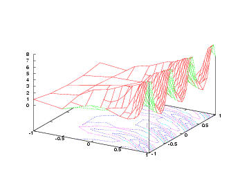
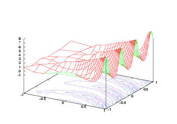
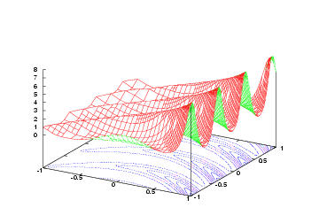
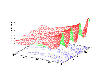
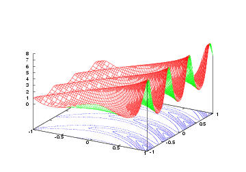
What surprises here is that the exact value is 1.59491554..., and that it is apparently surprisingly complicated to compute the solution even to only one per cent accuracy, although the solution is smooth (in fact infinitely often differentiable). This smoothness is shown in the graphical output generated by the program, here coarse grid and the first 9 refinement steps of the Kelly refinement indicator:
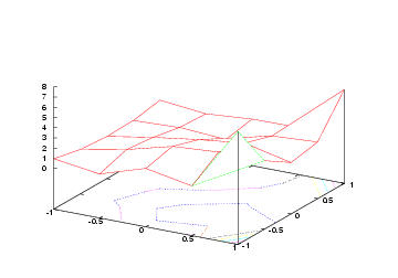 | 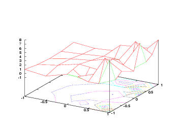 |
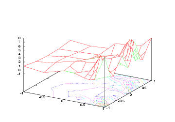 | 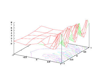 |
 |  |
 |  |
 |  |
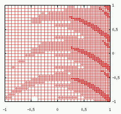
While we're already at watching pictures, this is the eighth grid, as viewed from top:
However, we are not yet finished with evaluation the point value computation. In fact, plotting the error e=|u(x_0)-u_h(x_0)| for the two refinement criteria yields the following picture:
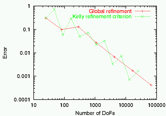
What is disturbing about this picture is that not only is the adaptive mesh refinement not better than global refinement as one would usually expect, it is even significantly worse since its convergence is irregular, preventing all extrapolation techniques when using the values of subsequent meshes! On the other hand, global refinement provides a perfect 1/N or h^{-2} convergence history and provides every opportunity to even improve on the point values by extrapolation. Global mesh refinement must therefore be considered superior in this example! This is even more surprising as the evaluation point is not somewhere in the left part where the mesh is coarse, but rather to the right and the adaptive refinement should refine the mesh around the evaluation point as well.
We thus close the discussion of this example program with a question:
What is wrong with adaptivity if it is not better than global refinement?
Exercise at the end of this example: There is a simple reason for the bad and irregular behavior of the adapted mesh solutions. It is simple to find out by looking at the mesh around the evaluation point in each of the steps - the data for this is in the output files of the program. An exercise would therefore be to modify the mesh refinement routine such that the problem (once you remark it) is avoided. The second exercise is to check whether the results are then better than global refinement, and if so if even a better order of convergence (in terms of the number of degrees of freedom) is achieved, or only by a better constant.
(Very brief answers for the impatient: at steps with larger errors, the mesh is not regular at the point of evaluation, i.e. some of the adjacent cells have hanging nodes; this destroys some superapproximation effects of which the globally refined mesh can profit. Answer 2: this quick hack
in the refinement function of the Kelly refinement class right before executing refinement would improve the results (exercise: what does the code do?), making them consistently better than global refinement. Behavior is still irregular, though, so no results about an order of convergence are possible.)
 1.8.17