 |
Reference documentation for deal.II version 9.2.0
|
 |
Reference documentation for deal.II version 9.2.0
|
This tutorial depends on step-34.
| Table of contents | |
|---|---|
This program was contributed by Andrea Bonito and M. Sebastian Pauletti, with editing and writing by Wolfgang Bangerth.
This material is based upon work supported by the National Science Foundation under Grant No. DMS-0914977. Any opinions, findings and conclusions or recommendations expressed in this material are those of the author(s) and do not necessarily reflect the views of the National Science Foundation (NSF).
In this example, we show how to solve a partial differential equation (PDE) on a codimension one surface \Gamma \subset \mathbb R^3 made of quadrilaterals, i.e. on a surface in 3d or a line in 2d. We focus on the following elliptic second order PDE
\begin{align*} -\Delta_\Gamma u &= f \qquad \text{on } \qquad \Gamma,\\ u &= g \qquad \text{on} \qquad \partial \Gamma, \end{align*}
which generalized the Laplace equation we have previously solved in several of the early tutorial programs. Our implementation is based on step-4. step-34 also solves problems on lower dimensional surfaces; however, there we only consider integral equations that do not involve derivatives on the solution variable, while here we actually have to investigate what it means to take derivatives of a function only defined on a (possibly curved) surface.
In order to define the above operator, we start by introducing some notations. Let \mathbf x_S:\hat S \rightarrow S be a parameterization of a surface S from a reference element \hat S \subset \mathbb R^2, i.e. each point \hat{\mathbf x}\in\hat S induces a point {\mathbf x}_S(\hat{\mathbf x}) \in S. Then let
G_S\dealcoloneq (D \mathbf{x}_S)^T \ D \mathbf{x}_S
denotes the corresponding first fundamental form, where D \mathbf{x}_S=\left(\frac{\partial x_{S,i}(\hat{\mathbf x})}{\partial \hat x_j}\right)_{ij} is the derivative (Jacobian) of the mapping. In the following, S will be either the entire surface \Gamma or, more convenient for the finite element method, any face S \in {\mathbb T}, where {\mathbb T} is a partition (triangulation) of \Gamma constituted of quadrilaterals. We are now in position to define the tangential gradient of a function v : S \rightarrow \mathbb R by
(\nabla_S v)\circ \mathbf x_S \dealcoloneq D \mathbf x_S \ G_S^{-1} \ \nabla (v \circ \mathbf x_S).
The surface Laplacian (also called the Laplace-Beltrami operator) is then defined as \Delta_S \dealcoloneq \nabla_S \cdot \nabla_S. Note that an alternate way to compute the surface gradient on smooth surfaces \Gamma is
\nabla_S v = \nabla \tilde v - \mathbf n (\mathbf n \cdot \nabla \tilde v),
where \tilde v is a "smooth" extension of v in a tubular neighborhood of \Gamma and \mathbf n is the normal of \Gamma. Since \Delta_S = \nabla_S \cdot \nabla_S, we deduce
\Delta_S v = \Delta \tilde v - \mathbf n^T \ D^2 \tilde v \ \mathbf n - (\mathbf n \cdot \nabla \tilde v) (\nabla \cdot \mathbf n - \mathbf n^T \ D \mathbf n \ \mathbf n ).
Worth mentioning, the term \nabla \cdot \mathbf n - \mathbf n \ D \mathbf n \ \mathbf n appearing in the above expression is the total curvature of the surface (sum of principal curvatures).
As usual, we are only interested in weak solutions for which we can use C^0 finite elements (rather than requiring C^1 continuity as for strong solutions). We therefore resort to the weak formulation
\int_\Gamma \nabla_\Gamma u \cdot \nabla_\Gamma v = \int_\Gamma f \ v \qquad \forall v \in H^1_0(\Gamma)
and take advantage of the partition {\mathbb T} to further write
\sum_{K\in {\mathbb T}}\int_K \nabla_{K} u \cdot \nabla_{K} v = \sum_{K\in {\mathbb T}} \int_K f \ v \qquad \forall v \in H^1_0(\Gamma).
Moreover, each integral in the above expression is computed in the reference element \hat K \dealcoloneq [0,1]^2 so that
\begin{align*} \int_{K} \nabla_{K} u \cdot \nabla_{K} v &= \int_{\hat K} \nabla (u \circ \mathbf x_K)^T G_K^{-1} (D \mathbf x_K)^T D \mathbf x_K G_K^{-1} \nabla (v \circ \mathbf x_K) \sqrt{\det (G_K)} \\ &= \int_{\hat K} \nabla (u \circ \mathbf x_K)^T G_K^{-1} \nabla (v \circ \mathbf x_K) \sqrt{\det (G_K)} \end{align*}
and
\int_{K} f \ v = \int_{\hat K} (f \circ \mathbf x_K) (v \circ \mathbf x_K) \sqrt{\det (G_K)}.
Finally, we use a quadrature formula defined by points \{p_l\}_{l=1}^N\subset \hat K and weights \{w_l\}_{l=1}^N \subset \mathbb R^+_* to evaluate the above integrals and obtain
\int_{K} \nabla_{K} u \cdot \nabla_{K} v \approx \sum_{l=1}^N (\nabla (u \circ \mathbf x_K)(p_l))^T G^{-1}(p_l) \nabla (v \circ \mathbf x_K) (p_l) \sqrt{\det (G(p_l))} \ w_l
and
\int_{K} f \ v \approx \sum_{l=1}^N (f \circ \mathbf x_K)(p_l) \ (v \circ \mathbf x_K)(p_l) \sqrt{\det (G(p_l))} \ w_l.
Fortunately, deal.II has already all the tools to compute the above expressions. In fact, they barely differ from the ways in which we solve the usual Laplacian, only requiring the surface coordinate mapping to be provided in the constructor of the FEValues class. This surface description given, in the codimension one surface case, the two routines FEValues::shape_grad and FEValues::JxW return
\begin{align*} \text{FEValues::shape\_grad}(i,l)&=D \mathbf x_K(p_l) G^{-1}(p_l)D(\varphi_i \circ \mathbf x_K) (p_l) \\ \text{FEValues::JxW}(l) &= \sqrt{\det (G(p_l))} \ w_l. \end{align*}
This provides exactly the terms we need for our computations.
On a more general note, details for the finite element approximation on surfaces can be found for instance in [Dziuk, in Partial differential equations and calculus of variations 1357, Lecture Notes in Math., 1988], [Demlow, SIAM J. Numer. Anal. 47(2), 2009] and [Bonito, Nochetto, and Pauletti, SIAM J. Numer. Anal. 48(5), 2010].
In general when you want to test numerically the accuracy and/or order of convergence of an algorithm you need to provide an exact solution. The usual trick is to pick a function that we want to be the solution, then apply the differential operator to it that defines a forcing term for the right hand side. This is what we do in this example. In the current case, the form of the domain is obviously also essential.
We produce one test case for a 2d problem and another one for 3d:
In 2d, let's choose as domain a half circle. On this domain, we choose the function u(\mathbf x)=-2x_1x_2 as the solution. To compute the right hand side, we have to compute the surface Laplacian of the solution function. There are (at least) two ways to do that. The first one is to project away the normal derivative as described above using the natural extension of u(\mathbf x) (still denoted by u) over \mathbb R^d, i.e. to compute
-\Delta_\Gamma u = \Delta u - \mathbf n^T \ D^2 u \ \mathbf n - (\mathbf n \cdot \nabla u)\ \kappa,
where \kappa is the total curvature of \Gamma. Since we are on the unit circle, \mathbf n=\mathbf x and \kappa = 1 so that
-\Delta_\Gamma u = -8 x_1x_2.
A somewhat simpler way, at least for the current case of a curve in two-dimensional space, is to note that we can map the interval t \in [0,\pi] onto the domain \Omega using the transformation \mathbf x(t)= \left(\begin{array}{c} \cos t \\ \sin t \end{array}\right). At position \mathbf x=\mathbf x(t), the value of the solution is then u(\mathbf x(t)) = -2\cos t \sin t. Taking into account that the transformation is length preserving, i.e. a segment of length dt is mapped onto a piece of curve of exactly the same length, the tangential Laplacian then satisfies
\begin{align*} \Delta_\Gamma u &= \frac{d^2}{dt^2}(-2\cos t \sin t) = -2 \frac{d}{dt}(-\sin^2 t + \cos^2 t) = -2 (-2 \sin t \cos t - 2 \cos t \sin t) \\ &= 8 \sin t \cos t \\ &= 8 x_1x_2, \end{align*}
which is of course the same result as we had above.
In the program, we will also compute the H^1 seminorm error of the solution. Since the solution function and its numerical approximation are only defined on the manifold, the obvious definition of this error functional is | e |_{H^1(\Gamma)} = | \nabla_\Gamma e |_{L_2(\Gamma)} = \left( \int_\Gamma | \nabla_\Gamma (u-u_h) |^2 \right)^{1/2}. This requires us to provide the tangential gradient \nabla_\Gamma u to the function VectorTools::integrate_difference (first introduced in step-7), which we will do by implementing the function Solution::gradient in the program below.
If you've read through step-4 and understand the discussion above of how solution and right hand side correspond to each other, you will be immediately familiar with this program as well. In fact, there are only two things that are of significance:
Mapping objects were already introduced in step-10 and step-11 and as explained there, there is usually not a whole lot you have to know about how they work as long as you have a working description of how the boundary looks. In essence, we will simply declare an appropriate object of type MappingQ that will automatically obtain the boundary description from the Triangulation. The mapping object will then be passed to the appropriate functions, and we will get a boundary description for half circles or half spheres that is predefined in the library.
The rest of the program follows closely step-4 and, as far as computing the error, step-7. Some aspects of this program, in particular the use of two template arguments on the classes Triangulation, DoFHandler, and similar, are already described in detail in step-34; you may wish to read through this tutorial program as well.
If you've read through step-4 and step-7, you will recognize that we have used all of the following include files there already. Consequently, we will not explain their meaning here again.
LaplaceBeltramiProblem class templateThis class is almost exactly similar to the LaplaceProblem class in step-4.
The essential differences are these:
spacedim, and introducing a constant dim equal to the dimensionality of the domain – here equal to spacedim-1.dim, and the other for the dimension of the embedding space, spacedim. This is exactly what we did in step-34, take a look there for a deeper explanation.Next, let us define the classes that describe the exact solution and the right hand sides of the problem. This is in analogy to step-4 and step-7 where we also defined such objects. Given the discussion in the introduction, the actual formulas should be self-explanatory. A point of interest may be how we define the value and gradient functions for the 2d and 3d cases separately, using explicit specializations of the general template. An alternative to doing it this way might have been to define the general template and have a switch statement (or a sequence of ifs) for each possible value of the spatial dimension.
LaplaceBeltramiProblem classThe rest of the program is actually quite unspectacular if you know step-4. Our first step is to define the constructor, setting the polynomial degree of the finite element and mapping, and associating the DoF handler to the triangulation:
The next step is to create the mesh, distribute degrees of freedom, and set up the various variables that describe the linear system. All of these steps are standard with the exception of how to create a mesh that describes a surface. We could generate a mesh for the domain we are interested in, generate a triangulation using a mesh generator, and read it in using the GridIn class. Or, as we do here, we generate the mesh using the facilities in the GridGenerator namespace.
In particular, what we're going to do is this (enclosed between the set of braces below): we generate a spacedim dimensional mesh for the half disk (in 2d) or half ball (in 3d), using the GridGenerator::half_hyper_ball function. This function sets the boundary indicators of all faces on the outside of the boundary to zero for the ones located on the perimeter of the disk/ball, and one on the straight part that splits the full disk/ball into two halves. The next step is the main point: The GridGenerator::extract_boundary_mesh function creates a mesh that consists of those cells that are the faces of the previous mesh, i.e. it describes the surface cells of the original (volume) mesh. However, we do not want all faces: only those on the perimeter of the disk or ball which carry boundary indicator zero; we can select these cells using a set of boundary indicators that we pass to GridGenerator::extract_boundary_mesh.
There is one point that needs to be mentioned. In order to refine a surface mesh appropriately if the manifold is curved (similarly to refining the faces of cells that are adjacent to a curved boundary), the triangulation has to have an object attached to it that describes where new vertices should be located. If you don't attach such a boundary object, they will be located halfway between existing vertices; this is appropriate if you have a domain with straight boundaries (e.g. a polygon) but not when, as here, the manifold has curvature. So for things to work properly, we need to attach a manifold object to our (surface) triangulation, in much the same way as we've already done in 1d for the boundary. We create such an object and attach it to the triangulation.
The final step in creating the mesh is to refine it a number of times. The rest of the function is the same as in previous tutorial programs.
The following is the central function of this program, assembling the matrix that corresponds to the surface Laplacian (Laplace-Beltrami operator). Maybe surprisingly, it actually looks exactly the same as for the regular Laplace operator discussed in, for example, step-4. The key is that the FEValues::shape_grad() function does the magic: It returns the surface gradient \nabla_K \phi_i(x_q) of the ith shape function at the qth quadrature point. The rest then does not need any changes either:
The next function is the one that solves the linear system. Here, too, no changes are necessary:
This is the function that generates graphical output from the solution. Most of it is boilerplate code, but there are two points worth pointing out:
This is the last piece of functionality: we want to compute the error in the numerical solution. It is a verbatim copy of the code previously shown and discussed in step-7. As mentioned in the introduction, the Solution class provides the (tangential) gradient of the solution. To avoid evaluating the error only a superconvergence points, we choose a quadrature rule of sufficiently high order.
The last function provides the top-level logic. Its contents are self-explanatory:
The remainder of the program is taken up by the main() function. It follows exactly the general layout first introduced in step-6 and used in all following tutorial programs:
When you run the program, the following output should be printed on screen:
Surface mesh has 1280 cells.
Surface mesh has 5185 degrees of freedom.
H1 error = 0.0217136
By playing around with the number of global refinements in the LaplaceBeltrami::make_grid_and_dofs function you increase or decrease mesh refinement. For example, doing one more refinement and only running the 3d surface problem yields the following output:
Surface mesh has 5120 cells.
Surface mesh has 20609 degrees of freedom.
H1 error = 0.00543481
This is what we expect: make the mesh size smaller by a factor of two and the error goes down by a factor of four (remember that we use bi-quadratic elements). The full sequence of errors from one to five refinements looks like this, neatly following the theoretically predicted pattern:
0.339438
0.0864385
0.0217136
0.00543481
0.00135913
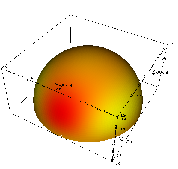
Finally, the program produces graphical output that we can visualize. Here is a plot of the results:

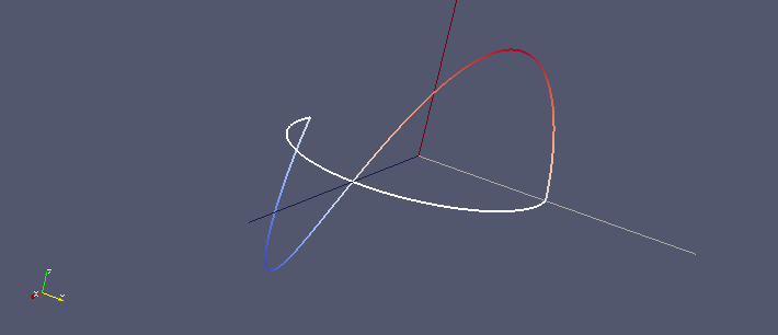
The program also works for 1d curves in 2d, not just 2d surfaces in 3d. You can test this by changing the template argument in main() like so:
The domain is a curve in 2d, and we can visualize the solution by using the third dimension (and color) to denote the value of the function u(x). This then looks like so (the white curve is the domain, the colored curve is the solution extruded into the third dimension, clearly showing the change in sign as the curve moves from one quadrant of the domain into the adjacent one):

Computing on surfaces only becomes interesting if the surface is more interesting than just a half sphere. To achieve this, deal.II can read meshes that describe surfaces through the usual GridIn class. Or, in case you have an analytic description, a simple mesh can sometimes be stretched and bent into a shape we are interested in.
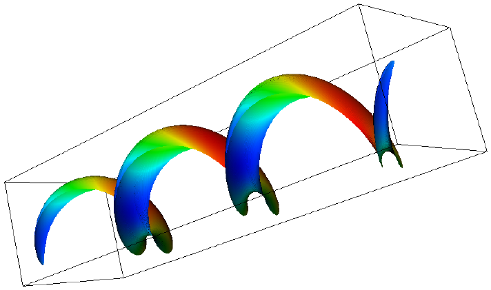
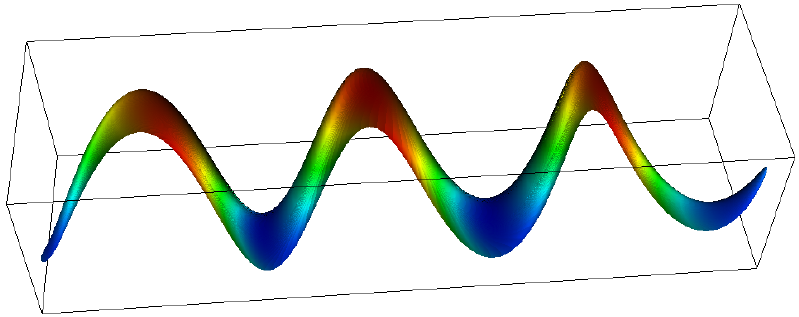
Let us consider a relatively simple example: we take the half sphere we used before, we stretch it by a factor of 10 in the z-direction, and then we jumble the x- and y-coordinates a bit. Let's show the computational domain and the solution first before we go into details of the implementation below:


The way to produce such a mesh is by using the GridTools::transform() function. It needs a way to transform each individual mesh point to a different position. Let us here use the following, rather simple function (remember: stretch in one direction, jumble in the other two):
If we followed the LaplaceBeltrami::make_grid_and_dofs function, we would extract the half spherical surface mesh as before, warp it into the shape we want, and refine as often as necessary. This is not quite as simple as we'd like here, though: refining requires that we have an appropriate manifold object attached to the triangulation that describes where new vertices of the mesh should be located upon refinement. I'm sure it's possible to describe this manifold in a not-too-complicated way by simply undoing the transformation above (yielding the spherical surface again), finding the location of a new point on the sphere, and then re-warping the result. But I'm a lazy person, and since doing this is not really the point here, let's just make our lives a bit easier: we'll extract the half sphere, refine it as often as necessary, get rid of the object that describes the manifold since we now no longer need it, and then finally warp the mesh. With the function above, this would look as follows:
Note that the only essential addition is the line marked with asterisks. It is worth pointing out one other thing here, though: because we detach the manifold description from the surface mesh, whenever we use a mapping object in the rest of the program, it has no curves boundary description to go on any more. Rather, it will have to use the implicit, FlatManifold class that is used on all parts of the domain not explicitly assigned a different manifold object. Consequently, whether we use MappingQ(2), MappingQ(15) or MappingQ1, each cell of our mesh will be mapped using a bilinear approximation.
All these drawbacks aside, the resulting pictures are still pretty. The only other differences to what's in step-38 is that we changed the right hand side to f(\mathbf x)=\sin x_3 and the boundary values (through the Solution class) to u(\mathbf x)|_{\partial\Omega}=\cos x_3. Of course, we now no longer know the exact solution, so the computation of the error at the end of LaplaceBeltrami::run will yield a meaningless number.
 1.8.17