This tutorial depends on step-7, step-39.
Note: A variant called step-12b of this tutorial exists, using MeshWorker and LocalIntegrators instead of assembling matrices using FEInterfaceValues as is done in this tutorial.
An example of an advection problem using the Discountinuous Galerkin method
Overview
This example is devoted to the discontinuous Galerkin method, or in short, the DG method. It includes the following topics.
-
Discretization of the linear advection equation with the DG method.
-
Assembling of jump terms and other expressions on the interface between cells using FEInterfaceValues.
-
Assembling of the system matrix using the MeshWorker::mesh_loop().
The particular concern of this program are the loops of DG methods. These turn out to be especially complex, primarily because for the face terms, we have to distinguish the cases of boundary, regular interior faces and interior faces with hanging nodes, respectively. The MeshWorker::mesh_loop() handles the complexity on iterating over cells and faces and allows specifying "workers" for the different cell and face terms. The integration of face terms itself, including on adaptively refined faces, is done using the FEInterfaceValues class.
The equation
The model problem solved in this example is the linear advection equation
\[ \nabla\cdot \left({\mathbf \beta} u\right)=0 \qquad\mbox{in }\Omega, \]
subject to the boundary conditions
\[ u=g\quad\mbox{on }\Gamma_-, \]
on the inflow part \(\Gamma_-\) of the boundary \(\Gamma=\partial\Omega\) of the domain. Here, \({\mathbf \beta}={\mathbf \beta}({\bf x})\) denotes a vector field, \(u\) the (scalar) solution function, \(g\) a boundary value function,
\[ \Gamma_- \dealcoloneq \{{\bf x}\in\Gamma, {\mathbf \beta}({\bf x})\cdot{\bf n}({\bf x})<0\} \]
the inflow part of the boundary of the domain and \({\bf n}\) denotes the unit outward normal to the boundary \(\Gamma\). This equation is the conservative version of the advection equation already considered in step-9 of this tutorial.
On each cell \(T\), we multiply by a test function \(v_h\) from the left and integrate by parts to get:
\[ \left( v_h, \nabla \cdot (\beta u_h) \right)_T = -(\nabla v_h, \beta u_h) + \int_\Gamma v_h u_h \beta \cdot n \]
When summing this expression over all cells \(T\), the boundary integral is done over all internal and external faces and as such there are three cases:
-
outer boundary on the inflow (we replace \(u_h\) by given \(g\)): \(\int_{\Gamma_-} v_h g \beta \cdot n\)
-
outer boundary on the outflow: \(\int_{\Gamma_+} v_h u_h \beta \cdot n\)
-
inner faces (integral from two sides turns into jump, we use the upwind velocity): \(\int_F [v_h] u_h^{\text{upwind}} \beta \cdot n\)
Here, the jump is defined as \([v] = v^+ - v^-\), where the superscripts refer to the left ('+') and right ('-') values at the face. The upwind value \(u^{\text{upwind}}\) is defined to be \(u^+\) if \(\beta \cdot n>0\) and \(u^-\) otherwise.
As a result, the mesh-dependent weak form reads:
\[ \sum_{T\in \mathbb T_h} -\bigl(\nabla \phi_i,{\mathbf \beta}\cdot \phi_j \bigr)_T + \sum_{F\in\mathbb F_h^i} \bigl< [\phi_i], \phi_j^{upwind} \beta\cdot \mathbf n\bigr>_{F} + \bigl<\phi_i, \phi_j \beta\cdot \mathbf n\bigr>_{\Gamma_+} = -\bigl<\phi_i, g \beta\cdot\mathbf n\bigr>_{\Gamma_-}. \]
Here, \(\mathbb T_h\) is the set of all active cells of the triangulation and \(\mathbb F_h^i\) is the set of all active interior faces. This formulation is known as the upwind discontinuous Galerkin method.
In order to implement this bilinear form, we need to compute the cell terms (first sum) using the usual way to achieve integration on a cell, the interface terms (second sum) using FEInterfaceValues, and the boundary terms (the other two terms). The summation of all those is done by MeshWorker::mesh_loop().
The test problem
We solve the advection equation on \(\Omega=[0,1]^2\) with \({\mathbf \beta}=\frac{1}{|x|}(-x_2, x_1)\) representing a circular counterclockwise flow field, and \(g=1\) on \({\bf x}\in\Gamma_-^1 := [0,0.5]\times\{0\}\) and \(g=0\) on \({\bf x}\in \Gamma_-\setminus \Gamma_-^1\).
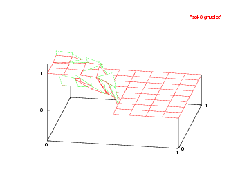
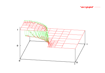
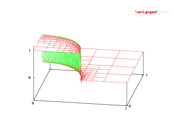
We solve on a sequence of meshes by refining the mesh adaptively by estimating the norm of the gradient on each cell. After solving on each mesh, we output the solution in vtk format and compute the \(L^\infty\) norm of the solution. As the exact solution is either 0 or 1, we can measure the magnitude of the overshoot of the numerical solution with this.
The commented program
The first few files have already been covered in previous examples and will thus not be further commented on:
Here the discontinuous finite elements are defined. They are used in the same way as all other finite elements, though – as you have seen in previous tutorial programs – there isn't much user interaction with finite element classes at all: they are passed to DoFHandler and FEValues objects, and that is about it.
This header is needed for FEInterfaceValues to compute integrals on interfaces:
We are going to use the simplest possible solver, called Richardson iteration, that represents a simple defect correction. This, in combination with a block SSOR preconditioner (defined in precondition_block.h), that uses the special block matrix structure of system matrices arising from DG discretizations.
We are going to use gradients as refinement indicator.
Finally, the new include file for using the mesh_loop from the MeshWorker framework
Like in all programs, we finish this section by including the needed C++ headers and declaring we want to use objects in the dealii namespace without prefix.
#include <iostream>
#include <fstream>
namespace Step12
{
Equation data
First, we define a class describing the inhomogeneous boundary data. Since only its values are used, we implement value_list(), but leave all other functions of Function undefined.
template <int dim>
class BoundaryValues :
public Function<dim>
{
public:
BoundaryValues() = default;
std::vector<double> & values,
const unsigned int component = 0) const override;
};
Given the flow direction, the inflow boundary of the unit square \([0,1]^2\) are the right and the lower boundaries. We prescribe discontinuous boundary values 1 and 0 on the x-axis and value 0 on the right boundary. The values of this function on the outflow boundaries will not be used within the DG scheme.
template <int dim>
void BoundaryValues<dim>::value_list(
const std::vector<
Point<dim>> &points,
std::vector<double> & values,
const unsigned int component) const
{
(void)component;
Assert(values.size() == points.size(),
for (unsigned int i = 0; i < values.size(); ++i)
{
if (points[i](0) < 0.5)
values[i] = 1.;
else
values[i] = 0.;
}
}
Finally, a function that computes and returns the wind field \(\beta=\beta(\mathbf x)\). As explained in the introduction, we will use a rotational field around the origin in 2d. In 3d, we simply leave the \(z\)-component unset (i.e., at zero), whereas the function can not be used in 1d in its current implementation:
template <int dim>
{
wind_field(0) = -p(1);
wind_field(1) = p(0);
wind_field /= wind_field.
norm();
return wind_field;
}
The ScratchData and CopyData classes
The following objects are the scratch and copy objects we use in the call to MeshWorker::mesh_loop(). The new object is the FEInterfaceValues object, that works similar to FEValues or FEFacesValues, except that it acts on an interface between two cells and allows us to assemble the interface terms in our weak form.
template <int dim>
struct ScratchData
{
const unsigned int quadrature_degree,
: fe_values(mapping, fe,
QGauss<dim>(quadrature_degree), update_flags)
, fe_interface_values(mapping,
fe,
QGauss<dim - 1>(quadrature_degree),
interface_update_flags)
{}
ScratchData(const ScratchData<dim> &scratch_data)
: fe_values(scratch_data.fe_values.get_mapping(),
scratch_data.fe_values.get_fe(),
scratch_data.fe_values.get_quadrature(),
scratch_data.fe_values.get_update_flags())
, fe_interface_values(
scratch_data.fe_values
.get_mapping(),
scratch_data.fe_values.get_fe(),
scratch_data.fe_interface_values.get_quadrature(),
scratch_data.fe_interface_values.get_update_flags())
{}
};
struct CopyDataFace
{
std::vector<types::global_dof_index> joint_dof_indices;
};
struct CopyData
{
std::vector<types::global_dof_index> local_dof_indices;
std::vector<CopyDataFace> face_data;
template <class Iterator>
{
cell_rhs.
reinit(dofs_per_cell);
local_dof_indices.resize(dofs_per_cell);
cell->get_dof_indices(local_dof_indices);
}
};
The AdvectionProblem class
After this preparations, we proceed with the main class of this program, called AdvectionProblem.
This should all be pretty familiar to you. Interesting details will only come up in the implementation of the assemble function.
template <int dim>
class AdvectionProblem
{
public:
AdvectionProblem();
private:
void setup_system();
void assemble_system();
void solve();
void refine_grid();
void output_results(const unsigned int cycle) const;
Furthermore we want to use DG elements.
The next four members represent the linear system to be solved. system_matrix and right_hand_side are generated by assemble_system(), the solution is computed in solve(). The sparsity_pattern is used to determine the location of nonzero elements in system_matrix.
We start with the constructor. The 1 in the constructor call of fe is the polynomial degree.
template <int dim>
AdvectionProblem<dim>::AdvectionProblem()
: mapping()
, fe(1)
{}
template <int dim>
void AdvectionProblem<dim>::setup_system()
{
In the function that sets up the usual finite element data structures, we first need to distribute the DoFs.
dof_handler.distribute_dofs(fe);
We start by generating the sparsity pattern. To this end, we first fill an intermediate object of type DynamicSparsityPattern with the couplings appearing in the system. After building the pattern, this object is copied to sparsity_pattern and can be discarded.
To build the sparsity pattern for DG discretizations, we can call the function analogue to DoFTools::make_sparsity_pattern, which is called DoFTools::make_flux_sparsity_pattern:
sparsity_pattern.copy_from(dsp);
Finally, we set up the structure of all components of the linear system.
system_matrix.reinit(sparsity_pattern);
solution.reinit(dof_handler.n_dofs());
right_hand_side.reinit(dof_handler.n_dofs());
}
The assemble_system function
Here we see the major difference to assembling by hand. Instead of writing loops over cells and faces, the logic is contained in the call to MeshWorker::mesh_loop() and we only need to specify what should happen on each cell, each boundary face, and each interior face. These three tasks are handled by the lambda functions inside the function below.
template <int dim>
void AdvectionProblem<dim>::assemble_system()
{
const BoundaryValues<dim> boundary_function;
This is the function that will be executed for each cell.
auto cell_worker = [&](
const Iterator & cell,
ScratchData<dim> &scratch_data,
CopyData & copy_data) {
const unsigned int n_dofs = scratch_data.fe_values.get_fe().dofs_per_cell;
copy_data.reinit(cell, n_dofs);
scratch_data.fe_values.reinit(cell);
const auto &q_points = scratch_data.fe_values.get_quadrature_points();
const std::vector<double> &JxW = fe_v.get_JxW_values();
We solve a homogeneous equation, thus no right hand side shows up in the cell term. What's left is integrating the matrix entries.
{
auto beta_q = beta(q_points[
point]);
for (unsigned int i = 0; i < n_dofs; ++i)
for (unsigned int j = 0; j < n_dofs; ++j)
{
copy_data.cell_matrix(i, j) +=
-beta_q
* fe_v.shape_grad(i,
point)
* fe_v.shape_value(j,
point)
}
}
};
This is the function called for boundary faces and consists of a normal integration using FEFaceValues. New is the logic to decide if the term goes into the system matrix (outflow) or the right-hand side (inflow).
auto boundary_worker = [&](
const Iterator & cell,
const unsigned int &face_no,
ScratchData<dim> & scratch_data,
CopyData & copy_data) {
scratch_data.fe_interface_values.reinit(cell, face_no);
scratch_data.fe_interface_values.get_fe_face_values(0);
const unsigned int n_facet_dofs = fe_face.
get_fe().n_dofs_per_cell();
std::vector<double> g(q_points.size());
boundary_function.value_list(q_points, g);
{
const double beta_dot_n = beta(q_points[
point]) * normals[
point];
if (beta_dot_n > 0)
{
for (unsigned int i = 0; i < n_facet_dofs; ++i)
for (unsigned int j = 0; j < n_facet_dofs; ++j)
copy_data.cell_matrix(i, j) +=
* beta_dot_n
}
else
for (unsigned int i = 0; i < n_facet_dofs; ++i)
* beta_dot_n
}
};
This is the function called on interior faces. The arguments specify cells, face and subface indices (for adaptive refinement). We just pass them along to the reinit() function of FEInterfaceValues.
auto face_worker = [&](
const Iterator & cell,
const unsigned int &f,
const unsigned int &sf,
const unsigned int &nf,
const unsigned int &nsf,
ScratchData<dim> & scratch_data,
CopyData & copy_data) {
fe_iv.
reinit(cell, f, sf, ncell, nf, nsf);
copy_data.face_data.emplace_back();
CopyDataFace ©_data_face = copy_data.face_data.back();
copy_data_face.cell_matrix.reinit(n_dofs, n_dofs);
for (unsigned int qpoint = 0; qpoint < q_points.size(); ++qpoint)
{
const double beta_dot_n = beta(q_points[qpoint]) * normals[qpoint];
for (unsigned int i = 0; i < n_dofs; ++i)
for (unsigned int j = 0; j < n_dofs; ++j)
copy_data_face.cell_matrix(i, j) +=
*
* beta_dot_n
* JxW[qpoint];
}
};
The following lambda function will handle copying the data from the cell and face assembly into the global matrix and right-hand side.
While we would not need an AffineConstraints object, because there are no hanging node constraints in DG discretizations, we use an empty object here as this allows us to use its copy_local_to_global functionality.
auto copier = [&](const CopyData &c) {
c.cell_rhs,
c.local_dof_indices,
system_matrix,
right_hand_side);
for (auto &cdf : c.face_data)
{
cdf.joint_dof_indices,
system_matrix);
}
};
const unsigned int n_gauss_points = dof_handler.get_fe().degree + 1;
ScratchData<dim> scratch_data(mapping, fe, n_gauss_points);
CopyData copy_data;
Here, we finally handle the assembly. We pass in ScratchData and CopyData objects, the lambda functions from above, an specify that we want to assemble interior faces once.
dof_handler.end(),
cell_worker,
copier,
scratch_data,
copy_data,
boundary_worker,
face_worker);
}
All the rest
For this simple problem we use the simplest possible solver, called Richardson iteration, that represents a simple defect correction. This, in combination with a block SSOR preconditioner, that uses the special block matrix structure of system matrices arising from DG discretizations. The size of these blocks are the number of DoFs per cell. Here, we use a SSOR preconditioning as we have not renumbered the DoFs according to the flow field. If the DoFs are renumbered in the downstream direction of the flow, then a block Gauss-Seidel preconditioner (see the PreconditionBlockSOR class with relaxation=1) does a much better job.
template <int dim>
void AdvectionProblem<dim>::solve()
{
Here we create the preconditioner,
then assign the matrix to it and set the right block size:
After these preparations we are ready to start the linear solver.
solver.solve(system_matrix, solution, right_hand_side, preconditioner);
std::cout << " Solver converged in " << solver_control.last_step()
<< " iterations." << std::endl;
}
We refine the grid according to a very simple refinement criterion, namely an approximation to the gradient of the solution. As here we consider the DG(1) method (i.e. we use piecewise bilinear shape functions) we could simply compute the gradients on each cell. But we do not want to base our refinement indicator on the gradients on each cell only, but want to base them also on jumps of the discontinuous solution function over faces between neighboring cells. The simplest way of doing that is to compute approximative gradients by difference quotients including the cell under consideration and its neighbors. This is done by the DerivativeApproximation class that computes the approximate gradients in a way similar to the GradientEstimation described in step-9 of this tutorial. In fact, the DerivativeApproximation class was developed following the GradientEstimation class of step-9. Relating to the discussion in step-9, here we consider \(h^{1+d/2}|\nabla_h u_h|\). Furthermore we note that we do not consider approximate second derivatives because solutions to the linear advection equation are in general not in \(H^2\) but only in \(H^1\) (or, to be more precise: in \(H^1_\beta\), i.e., the space of functions whose derivatives in direction \(\beta\) are square integrable).
template <int dim>
void AdvectionProblem<dim>::refine_grid()
{
The DerivativeApproximation class computes the gradients to float precision. This is sufficient as they are approximate and serve as refinement indicators only.
Now the approximate gradients are computed
dof_handler,
solution,
gradient_indicator);
and they are cell-wise scaled by the factor \(h^{1+d/2}\)
unsigned int cell_no = 0;
for (const auto &cell : dof_handler.active_cell_iterators())
gradient_indicator(cell_no++) *=
std::pow(cell->diameter(), 1 + 1.0 * dim / 2);
Finally they serve as refinement indicator.
gradient_indicator,
0.3,
0.1);
}
The output of this program consists of a vtk file of the adaptively refined grids and the numerical solutions. Finally, we also compute the L-infinity norm of the solution using VectorTools::integrate_difference().
template <int dim>
void AdvectionProblem<dim>::output_results(const unsigned int cycle) const
{
const std::string filename =
"solution-" +
std::to_string(cycle) +
".vtk";
std::cout << " Writing solution to <" << filename << ">" << std::endl;
std::ofstream output(filename);
{
solution,
values,
const double l_infty =
values,
std::cout << " L-infinity norm: " << l_infty << std::endl;
}
}
The following run function is similar to previous examples.
template <int dim>
{
for (unsigned int cycle = 0; cycle < 6; ++cycle)
{
std::cout << "Cycle " << cycle << std::endl;
if (cycle == 0)
{
}
else
refine_grid();
std::cout << " Number of active cells: "
setup_system();
std::cout << " Number of degrees of freedom: " << dof_handler.n_dofs()
<< std::endl;
assemble_system();
solve();
output_results(cycle);
}
}
}
The following main function is similar to previous examples as well, and need not be commented on.
int main()
{
try
{
Step12::AdvectionProblem<2> dgmethod;
dgmethod.run();
}
catch (std::exception &exc)
{
std::cerr << std::endl
<< std::endl
<< "----------------------------------------------------"
<< std::endl;
std::cerr << "Exception on processing: " << std::endl
<< exc.what() << std::endl
<< "Aborting!" << std::endl
<< "----------------------------------------------------"
<< std::endl;
return 1;
}
catch (...)
{
std::cerr << std::endl
<< std::endl
<< "----------------------------------------------------"
<< std::endl;
std::cerr << "Unknown exception!" << std::endl
<< "Aborting!" << std::endl
<< "----------------------------------------------------"
<< std::endl;
return 1;
}
return 0;
}
Results
The output of this program consist of the console output and solutions in vtk format:
Cycle 0
Number of active cells: 64
Number of degrees of freedom: 256
Solver converged in 4 iterations.
Writing solution to <solution-0.vtk>
Cycle 1
Number of active cells: 112
Number of degrees of freedom: 448
Solver converged in 9 iterations.
Writing solution to <solution-1.vtk>
Cycle 2
Number of active cells: 214
Number of degrees of freedom: 856
Solver converged in 16 iterations.
Writing solution to <solution-2.vtk>
Cycle 3
Number of active cells: 415
Number of degrees of freedom: 1660
Solver converged in 26 iterations.
Writing solution to <solution-3.vtk>
Cycle 4
Number of active cells: 796
Number of degrees of freedom: 3184
Solver converged in 44 iterations.
Writing solution to <solution-4.vtk>
Cycle 5
Number of active cells: 1561
Number of degrees of freedom: 6244
Solver converged in 81 iterations.
Writing solution to <solution-5.vtk>
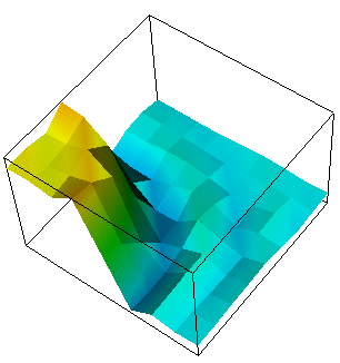
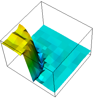
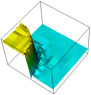
We show the solutions on the initial mesh, the mesh after two and after five adaptive refinement steps.
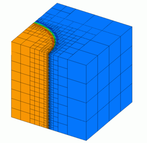
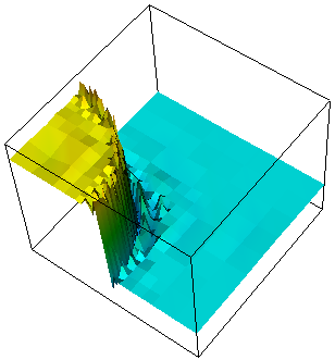
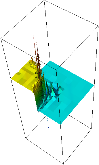
And finally we show a plot of a 3d computation.
Why use discontinuous elements
In this program we have used discontinuous elements. It is a legitimate question to ask why not simply use the normal, continuous ones. Of course, to everyone with a background in numerical methods, the answer is obvious: the continuous Galerkin (cG) method is not stable for the transport equation, unless one specifically adds stabilization terms. The DG method, however, is stable. Illustrating this with the current program is not very difficult; in fact, only the following minor modifications are necessary:
- Change the element to FE_Q instead of FE_DGQ.
- Add handling of hanging node constraints in exactly the same way as step-6.
- We need a different solver; the direct solver in step-29 is a convenient choice. An experienced deal.II user will be able to do this in less than 10 minutes.
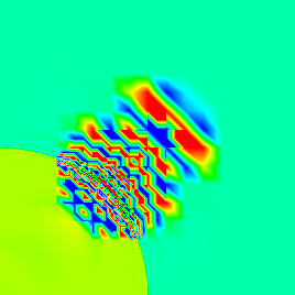
While the 2d solution has been shown above, containing a number of small spikes at the interface that are, however, stable in height under mesh refinement, results look much different when using a continuous element:
In refinement iteration 5, the image can't be plotted in a reasonable way any more as a 3d plot. We thus show a color plot with a range of \([-1,2]\) (the solution values of the exact solution lie in \([0,1]\), of course). In any case, it is clear that the continuous Galerkin solution exhibits oscillatory behavior that gets worse and worse as the mesh is refined more and more.
There are a number of strategies to stabilize the cG method, if one wants to use continuous elements for some reason. Discussing these methods is beyond the scope of this tutorial program; an interested reader could, for example, take a look at step-31.
Possibilities for extensions
Given that the exact solution is known in this case, one interesting avenue for further extensions would be to confirm the order of convergence for this program. In the current case, the solution is non-smooth, and so we can not expect to get a particularly high order of convergence, even if we used higher order elements. But even if the solution is smooth, the equation is not elliptic and so it is not immediately clear that we should obtain a convergence order that equals that of the optimal interpolation estimates (i.e. for example that we would get \(h^3\) convergence in the \(L^2\) norm by using quadratic elements).
In fact, for hyperbolic equations, theoretical predictions often indicate that the best one can hope for is an order one half below the interpolation estimate. For example, for the streamline diffusion method (an alternative method to the DG method used here to stabilize the solution of the transport equation), one can prove that for elements of degree \(p\), the order of convergence is \(p+\frac 12\) on arbitrary meshes. While the observed order is frequently \(p+1\) on uniformly refined meshes, one can construct so-called Peterson meshes on which the worse theoretical bound is actually attained. This should be relatively simple to verify, for example using the VectorTools::integrate_difference function.
A different direction is to observe that the solution of transport problems often has discontinuities and that therefore a mesh in which we bisect every cell in every coordinate direction may not be optimal. Rather, a better strategy would be to only cut cells in the direction parallel to the discontinuity. This is called anisotropic mesh refinement and is the subject of step-30.
The plain program
#include <iostream>
#include <fstream>
namespace Step12
{
template <int dim>
class BoundaryValues :
public Function<dim>
{
public:
BoundaryValues() = default;
virtual void value_list(
const std::vector<
Point<dim>> &points,
std::vector<double> & values,
const unsigned int component = 0) const override;
};
template <int dim>
void BoundaryValues<dim>::value_list(
const std::vector<
Point<dim>> &points,
std::vector<double> & values,
const unsigned int component) const
{
(void)component;
Assert(values.size() == points.size(),
for (unsigned int i = 0; i < values.size(); ++i)
{
if (points[i](0) < 0.5)
values[i] = 1.;
else
values[i] = 0.;
}
}
template <int dim>
{
wind_field(0) = -p(1);
wind_field(1) = p(0);
wind_field /= wind_field.
norm();
return wind_field;
}
template <int dim>
struct ScratchData
{
const unsigned int quadrature_degree,
: fe_values(mapping, fe,
QGauss<dim>(quadrature_degree), update_flags)
, fe_interface_values(mapping,
fe,
QGauss<dim - 1>(quadrature_degree),
interface_update_flags)
{}
ScratchData(const ScratchData<dim> &scratch_data)
: fe_values(scratch_data.fe_values.get_mapping(),
scratch_data.fe_values.get_fe(),
scratch_data.fe_values.get_quadrature(),
scratch_data.fe_values.get_update_flags())
, fe_interface_values(
scratch_data.fe_values
.get_mapping(),
scratch_data.fe_values.get_fe(),
scratch_data.fe_interface_values.get_quadrature(),
scratch_data.fe_interface_values.get_update_flags())
{}
};
struct CopyDataFace
{
std::vector<types::global_dof_index> joint_dof_indices;
};
struct CopyData
{
std::vector<types::global_dof_index> local_dof_indices;
std::vector<CopyDataFace> face_data;
template <class Iterator>
{
cell_rhs.
reinit(dofs_per_cell);
local_dof_indices.resize(dofs_per_cell);
cell->get_dof_indices(local_dof_indices);
}
};
template <int dim>
class AdvectionProblem
{
public:
AdvectionProblem();
private:
void setup_system();
void assemble_system();
void solve();
void refine_grid();
void output_results(const unsigned int cycle) const;
};
template <int dim>
AdvectionProblem<dim>::AdvectionProblem()
: mapping()
, fe(1)
{}
template <int dim>
void AdvectionProblem<dim>::setup_system()
{
dof_handler.distribute_dofs(fe);
sparsity_pattern.copy_from(dsp);
system_matrix.reinit(sparsity_pattern);
solution.reinit(dof_handler.n_dofs());
right_hand_side.reinit(dof_handler.n_dofs());
}
template <int dim>
void AdvectionProblem<dim>::assemble_system()
{
const BoundaryValues<dim> boundary_function;
auto cell_worker = [&](
const Iterator & cell,
ScratchData<dim> &scratch_data,
CopyData & copy_data) {
const unsigned int n_dofs = scratch_data.fe_values.get_fe().dofs_per_cell;
copy_data.reinit(cell, n_dofs);
scratch_data.fe_values.reinit(cell);
const auto &q_points = scratch_data.fe_values.get_quadrature_points();
const std::vector<double> &JxW = fe_v.get_JxW_values();
{
auto beta_q = beta(q_points[
point]);
for (unsigned int i = 0; i < n_dofs; ++i)
for (unsigned int j = 0; j < n_dofs; ++j)
{
copy_data.cell_matrix(i, j) +=
-beta_q
* fe_v.shape_grad(i,
point)
* fe_v.shape_value(j,
point)
}
}
};
auto boundary_worker = [&](
const Iterator & cell,
const unsigned int &face_no,
ScratchData<dim> & scratch_data,
CopyData & copy_data) {
scratch_data.fe_interface_values.reinit(cell, face_no);
scratch_data.fe_interface_values.get_fe_face_values(0);
const unsigned int n_facet_dofs = fe_face.
get_fe().n_dofs_per_cell();
std::vector<double> g(q_points.size());
boundary_function.value_list(q_points, g);
{
const double beta_dot_n = beta(q_points[
point]) * normals[
point];
if (beta_dot_n > 0)
{
for (unsigned int i = 0; i < n_facet_dofs; ++i)
for (unsigned int j = 0; j < n_facet_dofs; ++j)
copy_data.cell_matrix(i, j) +=
* beta_dot_n
}
else
for (unsigned int i = 0; i < n_facet_dofs; ++i)
* beta_dot_n
}
};
auto face_worker = [&](
const Iterator & cell,
const unsigned int &f,
const unsigned int &sf,
const unsigned int &nf,
const unsigned int &nsf,
ScratchData<dim> & scratch_data,
CopyData & copy_data) {
fe_iv.
reinit(cell, f, sf, ncell, nf, nsf);
copy_data.face_data.emplace_back();
CopyDataFace ©_data_face = copy_data.face_data.back();
copy_data_face.cell_matrix.reinit(n_dofs, n_dofs);
for (unsigned int qpoint = 0; qpoint < q_points.size(); ++qpoint)
{
const double beta_dot_n = beta(q_points[qpoint]) * normals[qpoint];
for (unsigned int i = 0; i < n_dofs; ++i)
for (unsigned int j = 0; j < n_dofs; ++j)
copy_data_face.cell_matrix(i, j) +=
*
* beta_dot_n
* JxW[qpoint];
}
};
auto copier = [&](const CopyData &c) {
c.cell_rhs,
c.local_dof_indices,
system_matrix,
right_hand_side);
for (auto &cdf : c.face_data)
{
cdf.joint_dof_indices,
system_matrix);
}
};
const unsigned int n_gauss_points = dof_handler.get_fe().degree + 1;
ScratchData<dim> scratch_data(mapping, fe, n_gauss_points);
CopyData copy_data;
dof_handler.end(),
cell_worker,
copier,
scratch_data,
copy_data,
boundary_worker,
face_worker);
}
template <int dim>
void AdvectionProblem<dim>::solve()
{
solver.solve(system_matrix, solution, right_hand_side, preconditioner);
std::cout << " Solver converged in " << solver_control.last_step()
<< " iterations." << std::endl;
}
template <int dim>
void AdvectionProblem<dim>::refine_grid()
{
Vector<float> gradient_indicator(
triangulation.n_active_cells());
dof_handler,
solution,
gradient_indicator);
unsigned int cell_no = 0;
for (const auto &cell : dof_handler.active_cell_iterators())
gradient_indicator(cell_no++) *=
std::pow(cell->diameter(), 1 + 1.0 * dim / 2);
gradient_indicator,
0.3,
0.1);
}
template <int dim>
void AdvectionProblem<dim>::output_results(const unsigned int cycle) const
{
const std::string filename =
"solution-" +
std::to_string(cycle) +
".vtk";
std::cout << " Writing solution to <" << filename << ">" << std::endl;
std::ofstream output(filename);
{
solution,
values,
const double l_infty =
values,
std::cout << " L-infinity norm: " << l_infty << std::endl;
}
}
template <int dim>
{
for (unsigned int cycle = 0; cycle < 6; ++cycle)
{
std::cout << "Cycle " << cycle << std::endl;
if (cycle == 0)
{
}
else
refine_grid();
std::cout << " Number of active cells: "
setup_system();
std::cout << " Number of degrees of freedom: " << dof_handler.n_dofs()
<< std::endl;
assemble_system();
solve();
output_results(cycle);
}
}
}
int main()
{
try
{
Step12::AdvectionProblem<2> dgmethod;
dgmethod.run();
}
catch (std::exception &exc)
{
std::cerr << std::endl
<< std::endl
<< "----------------------------------------------------"
<< std::endl;
std::cerr << "Exception on processing: " << std::endl
<< exc.what() << std::endl
<< "Aborting!" << std::endl
<< "----------------------------------------------------"
<< std::endl;
return 1;
}
catch (...)
{
std::cerr << std::endl
<< std::endl
<< "----------------------------------------------------"
<< std::endl;
std::cerr << "Unknown exception!" << std::endl
<< "Aborting!" << std::endl
<< "----------------------------------------------------"
<< std::endl;
return 1;
}
return 0;
}


 1.8.17