 |
Reference documentation for deal.II version 9.1.1
|
 |
Reference documentation for deal.II version 9.1.1
|
This tutorial depends on step-8, step-18.
This program was contributed by Jean-Paul Pelteret and Andrew McBride.
This material is based upon work supported by the German Science Foundation (Deutsche Forschungsgemeinschaft, DFG), grant STE 544/39-1, and the National Research Foundation of South Africa.
The subject of this tutorial is nonlinear solid mechanics. Classical single-field approaches (see e.g. step-18) can not correctly describe the response of quasi-incompressible materials. The response is overly stiff; a phenomenon known as locking. Locking problems can be circumvented using a variety of alternative strategies. One such strategy is the three-field formulation. It is used here to model the three-dimensional, fully-nonlinear (geometrical and material) response of an isotropic continuum body. The material response is approximated as hyperelastic. Additionally, the three-field formulation employed is valid for quasi-incompressible as well as compressible materials.
The objective of this presentation is to provide a basis for using deal.II for problems in nonlinear solid mechanics. The linear problem was addressed in step-8. A non-standard, hypoelastic-type form of the geometrically nonlinear problem was partially considered in step-18: a rate form of the linearised constitutive relations is used and the problem domain evolves with the motion. Important concepts surrounding the nonlinear kinematics are absent in the theory and implementation. step-18 does, however, describe many of the key concepts to implement elasticity within the framework of deal.II.
We begin with a crash-course in nonlinear kinematics. For the sake of simplicity, we restrict our attention to the quasi-static problem. Thereafter, various key stress measures are introduced and the constitutive model described. We then describe the three-field formulation in detail prior to explaining the structure of the class used to manage the material. The setup of the example problem is then presented.
The three-field formulation implemented here was pioneered by Simo et al. (1985) and is known as the mixed Jacobian-pressure formulation. Important related contributions include those by Simo and Taylor (1991), and Miehe (1994). The notation adopted here draws heavily on the excellent overview of the theoretical aspects of nonlinear solid mechanics by Holzapfel (2001). A nice overview of issues pertaining to incompressible elasticity (at small strains) is given in Hughes (2000).
An example where this three-field formulation is used in a coupled problem is documented in
One can think of fourth-order tensors as linear operators mapping second-order tensors (matrices) onto themselves in much the same way as matrices map vectors onto vectors. There are various fourth-order unit tensors that will be required in the forthcoming presentation. The fourth-order unit tensors \(\mathcal{I}\) and \(\overline{\mathcal{I}}\) are defined by
\[ \mathbf{A} = \mathcal{I}:\mathbf{A} \qquad \text{and} \qquad \mathbf{A}^T = \overline{\mathcal{I}}:\mathbf{A} \, . \]
Note \(\mathcal{I} \neq \overline{\mathcal{I}}^T\). Furthermore, we define the symmetric and skew-symmetric fourth-order unit tensors by
\[ \mathcal{S} \dealcoloneq \dfrac{1}{2}[\mathcal{I} + \overline{\mathcal{I}}] \qquad \text{and} \qquad \mathcal{W} \dealcoloneq \dfrac{1}{2}[\mathcal{I} - \overline{\mathcal{I}}] \, , \]
such that
\[ \dfrac{1}{2}[\mathbf{A} + \mathbf{A}^T] = \mathcal{S}:\mathbf{A} \qquad \text{and} \qquad \dfrac{1}{2}[\mathbf{A} - \mathbf{A}^T] = \mathcal{W}:\mathbf{A} \, . \]
The fourth-order SymmetricTensor returned by identity_tensor() is \(\mathcal{S}\).
Let the time domain be denoted \(\mathbb{T} = [0,T_{\textrm{end}}]\), where \(t \in \mathbb{T}\) and \(T_{\textrm{end}}\) is the total problem duration. Consider a continuum body that occupies the reference configuration \(\Omega_0\) at time \(t=0\). Particles in the reference configuration are identified by the position vector \(\mathbf{X}\). The configuration of the body at a later time \(t>0\) is termed the current configuration, denoted \(\Omega\), with particles identified by the vector \(\mathbf{x}\). The nonlinear map between the reference and current configurations, denoted \(\boldsymbol{\varphi}\), acts as follows:
\[ \mathbf{x} = \boldsymbol{\varphi}(\mathbf{X},t) \, . \]
The material description of the displacement of a particle is defined by
\[ \mathbf{U}(\mathbf{X},t) = \mathbf{x}(\mathbf{X},t) - \mathbf{X} \, . \]
The deformation gradient \(\mathbf{F}\) is defined as the material gradient of the motion:
\[ \mathbf{F}(\mathbf{X},t) \dealcoloneq \dfrac{\partial \boldsymbol{\varphi}(\mathbf{X},t)}{\partial \mathbf{X}} = \textrm{Grad}\ \mathbf{x}(\mathbf{X},t) = \mathbf{I} + \textrm{Grad}\ \mathbf{U} \, . \]
The determinant of the of the deformation gradient \(J(\mathbf{X},t) \dealcoloneq \textrm{det}\ \mathbf{F}(\mathbf{X},t) > 0\) maps corresponding volume elements in the reference and current configurations, denoted \(\textrm{d}V\) and \(\textrm{d}v\), respectively, as
\[ \textrm{d}v = J(\mathbf{X},t)\; \textrm{d}V \, . \]
Two important measures of the deformation in terms of the spatial and material coordinates are the left and right Cauchy-Green tensors, respectively, and denoted \(\mathbf{b} \dealcoloneq \mathbf{F}\mathbf{F}^T\) and \(\mathbf{C} \dealcoloneq \mathbf{F}^T\mathbf{F}\). They are both symmetric and positive definite.
The Green-Lagrange strain tensor is defined by
\[ \mathbf{E} \dealcoloneq \frac{1}{2}[\mathbf{C} - \mathbf{I} ] = \underbrace{\frac{1}{2}[\textrm{Grad}^T \mathbf{U} + \textrm{Grad}\mathbf{U}]}_{\boldsymbol{\varepsilon}} + \frac{1}{2}[\textrm{Grad}^T\ \mathbf{U}][\textrm{Grad}\ \mathbf{U}] \, . \]
If the assumption of infinitesimal deformations is made, then the second term on the right can be neglected, and \(\boldsymbol{\varepsilon}\) (the linearised strain tensor) is the only component of the strain tensor. This assumption is, looking at the setup of the problem, not valid in step-18, making the use of the linearized \(\boldsymbol{\varepsilon}\) as the strain measure in that tutorial program questionable.
In order to handle the different response that materials exhibit when subjected to bulk and shear type deformations we consider the following decomposition of the deformation gradient \(\mathbf{F}\) and the left Cauchy-Green tensor \(\mathbf{b}\) into volume-changing (volumetric) and volume-preserving (isochoric) parts:
\[ \mathbf{F} = (J^{1/3}\mathbf{I})\overline{\mathbf{F}} \qquad \text{and} \qquad \mathbf{b} = (J^{2/3}\mathbf{I})\overline{\mathbf{F}}\,\overline{\mathbf{F}}^T = (J^{2/3}\mathbf{I})\overline{\mathbf{b}} \, . \]
Clearly, \(\textrm{det}\ \mathbf{F} = \textrm{det}\ (J^{1/3}\mathbf{I}) = J\).
The spatial velocity field is denoted \(\mathbf{v}(\mathbf{x},t)\). The derivative of the spatial velocity field with respect to the spatial coordinates gives the spatial velocity gradient \(\mathbf{l}(\mathbf{x},t)\), that is
\[ \mathbf{l}(\mathbf{x},t) \dealcoloneq \dfrac{\partial \mathbf{v}(\mathbf{x},t)}{\partial \mathbf{x}} = \textrm{grad}\ \mathbf{v}(\mathbf{x},t) \, , \]
where \(\textrm{grad} \{\bullet \} = \frac{\partial \{ \bullet \} }{ \partial \mathbf{x}} = \frac{\partial \{ \bullet \} }{ \partial \mathbf{X}}\frac{\partial \mathbf{X} }{ \partial \mathbf{x}} = \textrm{Grad} \{ \bullet \} \mathbf{F}^{-1}\).
Cauchy's stress theorem equates the Cauchy traction \(\mathbf{t}\) acting on an infinitesimal surface element in the current configuration \(\mathrm{d}a\) to the product of the Cauchy stress tensor \(\boldsymbol{\sigma}\) (a spatial quantity) and the outward unit normal to the surface \(\mathbf{n}\) as
\[ \mathbf{t}(\mathbf{x},t, \mathbf{n}) = \boldsymbol{\sigma}\mathbf{n} \, . \]
The Cauchy stress is symmetric. Similarly, the first Piola-Kirchhoff traction \(\mathbf{T}\) which acts on an infinitesimal surface element in the reference configuration \(\mathrm{d}A\) is the product of the first Piola-Kirchhoff stress tensor \(\mathbf{P}\) (a two-point tensor) and the outward unit normal to the surface \(\mathbf{N}\) as
\[ \mathbf{T}(\mathbf{X},t, \mathbf{N}) = \mathbf{P}\mathbf{N} \, . \]
The Cauchy traction \(\mathbf{t}\) and the first Piola-Kirchhoff traction \(\mathbf{T}\) are related as
\[ \mathbf{t}\mathrm{d}a = \mathbf{T}\mathrm{d}A \, . \]
This can be demonstrated using Nanson's formula.
The first Piola-Kirchhoff stress tensor is related to the Cauchy stress as
\[ \mathbf{P} = J \boldsymbol{\sigma}\mathbf{F}^{-T} \, . \]
Further important stress measures are the (spatial) Kirchhoff stress \(\boldsymbol{\tau} = J \boldsymbol{\sigma}\) and the (referential) second Piola-Kirchhoff stress \(\mathbf{S} = {\mathbf{F}}^{-1} \boldsymbol{\tau} {\mathbf{F}}^{-T}\).
Push-forward and pull-back operators allow one to transform various measures between the material and spatial settings. The stress measures used here are contravariant, while the strain measures are covariant.
The push-forward and-pull back operations for second-order covariant tensors \((\bullet)^{\text{cov}}\) are respectively given by:
\[ \chi_{*}(\bullet)^{\text{cov}} \dealcoloneq \mathbf{F}^{-T} (\bullet)^{\text{cov}} \mathbf{F}^{-1} \qquad \text{and} \qquad \chi^{-1}_{*}(\bullet)^{\text{cov}} \dealcoloneq \mathbf{F}^{T} (\bullet)^{\text{cov}} \mathbf{F} \, . \]
The push-forward and pull back operations for second-order contravariant tensors \((\bullet)^{\text{con}}\) are respectively given by:
\[ \chi_{*}(\bullet)^{\text{con}} \dealcoloneq \mathbf{F} (\bullet)^{\text{con}} \mathbf{F}^T \qquad \text{and} \qquad \chi^{-1}_{*}(\bullet)^{\text{con}} \dealcoloneq \mathbf{F}^{-1} (\bullet)^{\text{con}} \mathbf{F}^{-T} \, . \]
For example \(\boldsymbol{\tau} = \chi_{*}(\mathbf{S})\).
A hyperelastic material response is governed by a Helmholtz free energy function \(\Psi = \Psi(\mathbf{F}) = \Psi(\mathbf{C}) = \Psi(\mathbf{b})\) which serves as a potential for the stress. For example, if the Helmholtz free energy depends on the right Cauchy-Green tensor \(\mathbf{C}\) then the isotropic hyperelastic response is
\[ \mathbf{S} = 2 \dfrac{\partial \Psi(\mathbf{C})}{\partial \mathbf{C}} \, . \]
If the Helmholtz free energy depends on the left Cauchy-Green tensor \(\mathbf{b}\) then the isotropic hyperelastic response is
\[ \boldsymbol{\tau} = 2 \dfrac{\partial \Psi(\mathbf{b})}{\partial \mathbf{b}} \mathbf{b} = 2 \mathbf{b} \dfrac{\partial \Psi(\mathbf{b})}{\partial \mathbf{b}} \, . \]
Following the multiplicative decomposition of the deformation gradient, the Helmholtz free energy can be decomposed as
\[ \Psi(\mathbf{b}) = \Psi_{\text{vol}}(J) + \Psi_{\text{iso}}(\overline{\mathbf{b}}) \, . \]
Similarly, the Kirchhoff stress can be decomposed into volumetric and isochoric parts as \(\boldsymbol{\tau} = \boldsymbol{\tau}_{\text{vol}} + \boldsymbol{\tau}_{\text{iso}}\) where:
\begin{align*} \boldsymbol{\tau}_{\text{vol}} &= 2 \mathbf{b} \dfrac{\partial \Psi_{\textrm{vol}}(J)}{\partial \mathbf{b}} \\ &= p J\mathbf{I} \, , \\ \boldsymbol{\tau}_{\text{iso}} &= 2 \mathbf{b} \dfrac{\partial \Psi_{\textrm{iso}} (\overline{\mathbf{b}})}{\partial \mathbf{b}} \\ &= \underbrace{( \mathcal{I} - \dfrac{1}{3} \mathbf{I} \otimes \mathbf{I})}_{\mathbb{P}} : \overline{\boldsymbol{\tau}} \, , \end{align*}
where \(p \dealcoloneq \dfrac{\partial \Psi_{\text{vol}}(J)}{\partial J}\) is the pressure response. \(\mathbb{P}\) is the projection tensor which provides the deviatoric operator in the Eulerian setting. The fictitious Kirchhoff stress tensor \(\overline{\boldsymbol{\tau}}\) is defined by
\[ \overline{\boldsymbol{\tau}} \dealcoloneq 2 \overline{\mathbf{b}} \dfrac{\partial \Psi_{\textrm{iso}}(\overline{\mathbf{b}})}{\partial \overline{\mathbf{b}}} \, . \]
The Helmholtz free energy corresponding to a compressible neo-Hookean material is given by
\[ \Psi \equiv \underbrace{\kappa [ \mathcal{G}(J) ] }_{\Psi_{\textrm{vol}}(J)} + \underbrace{\bigl[c_1 [ \overline{I}_1 - 3] \bigr]}_{\Psi_{\text{iso}}(\overline{\mathbf{b}})} \, , \]
where \(\kappa \dealcoloneq \lambda + 2/3 \mu\) is the bulk modulus ( \(\lambda\) and \(\mu\) are the Lame parameters) and \(\overline{I}_1 \dealcoloneq \textrm{tr}\ \overline{\mathbf{b}}\). The function \(\mathcal{G}(J)\) is required to be strictly convex and satisfy the condition \(\mathcal{G}(1) = 0\), among others, see Holzapfel (2001) for further details. In this work \(\mathcal{G} \dealcoloneq \frac{1}{4} [ J^2 - 1 - 2\textrm{ln}J ]\).
Incompressibility imposes the isochoric constraint that \(J=1\) for all motions \(\boldsymbol{\varphi}\). The Helmholtz free energy corresponding to an incompressible neo-Hookean material is given by
\[ \Psi \equiv \underbrace{\bigl[ c_1 [ I_1 - 3] \bigr] }_{\Psi_{\textrm{iso}}(\mathbf{b})} \, , \]
where \( I_1 \dealcoloneq \textrm{tr}\mathbf{b} \). Thus, the incompressible response is obtained by removing the volumetric component from the compressible free energy and enforcing \(J=1\).
We will use a Newton-Raphson strategy to solve the nonlinear boundary value problem. Thus, we will need to linearise the constitutive relations.
The fourth-order elasticity tensor in the material description is defined by
\[ \mathfrak{C} = 2\dfrac{\partial \mathbf{S}(\mathbf{C})}{\partial \mathbf{C}} = 4\dfrac{\partial^2 \Psi(\mathbf{C})}{\partial \mathbf{C} \partial \mathbf{C}} \, . \]
The fourth-order elasticity tensor in the spatial description \(\mathfrak{c}\) is obtained from the push-forward of \(\mathfrak{C}\) as
\[ \mathfrak{c} = J^{-1} \chi_{*}(\mathfrak{C}) \qquad \text{and thus} \qquad J\mathfrak{c} = 4 \mathbf{b} \dfrac{\partial^2 \Psi(\mathbf{b})} {\partial \mathbf{b} \partial \mathbf{b}} \mathbf{b} \, . \]
The fourth-order elasticity tensors (for hyperelastic materials) possess both major and minor symmetries.
The fourth-order spatial elasticity tensor can be written in the following decoupled form:
\[ \mathfrak{c} = \mathfrak{c}_{\text{vol}} + \mathfrak{c}_{\text{iso}} \, , \]
where
\begin{align*} J \mathfrak{c}_{\text{vol}} &= 4 \mathbf{b} \dfrac{\partial^2 \Psi_{\text{vol}}(J)} {\partial \mathbf{b} \partial \mathbf{b}} \mathbf{b} \\ &= J[\widehat{p}\, \mathbf{I} \otimes \mathbf{I} - 2p \mathcal{I}] \qquad \text{where} \qquad \widehat{p} \dealcoloneq p + \dfrac{\textrm{d} p}{\textrm{d}J} \, , \\ J \mathfrak{c}_{\text{iso}} &= 4 \mathbf{b} \dfrac{\partial^2 \Psi_{\text{iso}}(\overline{\mathbf{b}})} {\partial \mathbf{b} \partial \mathbf{b}} \mathbf{b} \\ &= \mathbb{P} : \mathfrak{\overline{c}} : \mathbb{P} + \dfrac{2}{3}[\overline{\boldsymbol{\tau}}:\mathbf{I}]\mathbb{P} - \dfrac{2}{3}[ \mathbf{I}\otimes\boldsymbol{\tau}_{\text{iso}} + \boldsymbol{\tau}_{\text{iso}} \otimes \mathbf{I} ] \, , \end{align*}
where the fictitious elasticity tensor \(\overline{\mathfrak{c}}\) in the spatial description is defined by
\[ \overline{\mathfrak{c}} = 4 \overline{\mathbf{b}} \dfrac{ \partial^2 \Psi_{\textrm{iso}}(\overline{\mathbf{b}})} {\partial \overline{\mathbf{b}} \partial \overline{\mathbf{b}}} \overline{\mathbf{b}} \, . \]
The total potential energy of the system \(\Pi\) is the sum of the internal and external potential energies, denoted \(\Pi_{\textrm{int}}\) and \(\Pi_{\textrm{ext}}\), respectively. We wish to find the equilibrium configuration by minimising the potential energy.
As mentioned above, we adopt a three-field formulation. We denote the set of primary unknowns by \(\mathbf{\Xi} \dealcoloneq \{ \mathbf{u}, \widetilde{p}, \widetilde{J} \}\). The independent kinematic variable \(\widetilde{J}\) enters the formulation as a constraint on \(J\) enforced by the Lagrange multiplier \(\widetilde{p}\) (the pressure, as we shall see).
The three-field variational principle used here is given by
\[ \Pi(\mathbf{\Xi}) \dealcoloneq \int_\Omega \bigl[ \Psi_{\textrm{vol}}(\widetilde{J}) + \widetilde{p}\,[J(\mathbf{u}) - \widetilde{J}] + \Psi_{\textrm{iso}}(\overline{\mathbf{b}}(\mathbf{u})) \bigr] \textrm{d}v + \Pi_{\textrm{ext}} \, , \]
where the external potential is defined by
\[ \Pi_{\textrm{ext}} = - \int_\Omega \mathbf{b}^\text{p} \cdot \mathbf{u}~\textrm{d}v - \int_{\partial \Omega_{\sigma}} \mathbf{t}^\text{p} \cdot \mathbf{u}~\textrm{d}a \, . \]
The boundary of the current configuration \(\partial \Omega\) is composed into two parts as \(\partial \Omega = \partial \Omega_{\mathbf{u}} \cup \partial \Omega_{\sigma}\), where \(\partial \Omega_{\mathbf{u}} \cap \partial \Omega_{\boldsymbol{\sigma}} = \emptyset\). The prescribed Cauchy traction, denoted \(\mathbf{t}^\text{p}\), is applied to \( \partial \Omega_{\boldsymbol{\sigma}}\) while the motion is prescribed on the remaining portion of the boundary \(\partial \Omega_{\mathbf{u}}\). The body force per unit current volume is denoted \(\mathbf{b}^\text{p}\).
The stationarity of the potential follows as
\begin{align*} R(\mathbf\Xi;\delta \mathbf{\Xi}) &= D_{\delta \mathbf{\Xi}}\Pi(\mathbf{\Xi}) \\ &= \dfrac{\partial \Pi(\mathbf{\Xi})}{\partial \mathbf{u}} \cdot \delta \mathbf{u} + \dfrac{\partial \Pi(\mathbf{\Xi})}{\partial \widetilde{p}} \delta \widetilde{p} + \dfrac{\partial \Pi(\mathbf{\Xi})}{\partial \widetilde{J}} \delta \tilde{J} \\ &= \int_{\Omega_0} \left[ \textrm{grad}\ \delta\mathbf{u} : [ \underbrace{[\widetilde{p} J \mathbf{I}]}_{\equiv \boldsymbol{\tau}_{\textrm{vol}}} + \boldsymbol{\tau}_{\textrm{iso}}] + \delta \widetilde{p}\, [ J(\mathbf{u}) - \widetilde{J}] + \delta \widetilde{J}\left[ \dfrac{\textrm{d} \Psi_{\textrm{vol}}(\widetilde{J})}{\textrm{d} \widetilde{J}} -\widetilde{p}\right] \right]~\textrm{d}V \\ &\quad - \int_{\Omega_0} \delta \mathbf{u} \cdot \mathbf{B}^\text{p}~\textrm{d}V - \int_{\partial \Omega_{0,\boldsymbol{\sigma}}} \delta \mathbf{u} \cdot \mathbf{T}^\text{p}~\textrm{d}A \\ &=0 \, , \end{align*}
for all virtual displacements \(\delta \mathbf{u} \in H^1(\Omega)\) subject to the constraint that \(\delta \mathbf{u} = \mathbf{0}\) on \(\partial \Omega_{\mathbf{u}}\), and all virtual pressures \(\delta \widetilde{p} \in L^2(\Omega)\) and virtual dilatations \(\delta \widetilde{J} \in L^2(\Omega)\).
One should note that the definitions of the volumetric Kirchhoff stress in the three field formulation \(\boldsymbol{\tau}_{\textrm{vol}} \equiv \widetilde{p} J \mathbf{I}\) and the subsequent volumetric tangent differs slightly from the general form given in the section on hyperelastic materials where \(\boldsymbol{\tau}_{\textrm{vol}} \equiv p J\mathbf{I}\). This is because the pressure \(\widetilde{p}\) is now a primary field as opposed to a constitutively derived quantity. One needs to carefully distinguish between the primary fields and those obtained from the constitutive relations.
The Euler-Lagrange equations corresponding to the residual are:
\begin{align*} &\textrm{div}\ \boldsymbol{\sigma} + \mathbf{b}^\text{p} = \mathbf{0} && \textrm{[equilibrium]} \\ &J(\mathbf{u}) = \widetilde{J} && \textrm{[dilatation]} \\ &\widetilde{p} = \dfrac{\textrm{d} \Psi_{\textrm{vol}}(\widetilde{J})}{\textrm{d} \widetilde{J}} && \textrm{[pressure]} \, . \end{align*}
The first equation is the (quasi-static) equilibrium equation in the spatial setting. The second is the constraint that \(J(\mathbf{u}) = \widetilde{J}\). The third is the definition of the pressure \(\widetilde{p}\).
\begin{align*} \int_{\Omega}\delta \mathbf{u} \cdot [\textrm{div}\ \boldsymbol{\sigma} + \mathbf{b}^\text{p}]~\mathrm{d}v &= \int_{\Omega} [-\mathrm{grad}\delta \mathbf{u}:\boldsymbol{\sigma} + \delta \mathbf{u} \cdot\mathbf{b}^\text{p}]~\mathrm{d}v + \int_{\partial \Omega} \delta \mathbf{u} \cdot \mathbf{t}^\text{p}~\mathrm{d}a \\ &= - \int_{\Omega_0} \mathrm{grad}\delta \mathbf{u}:\boldsymbol{\tau}~\mathrm{d}V + \int_{\Omega_0} \delta \mathbf{u} \cdot J\mathbf{b}^\text{p}~\mathrm{d}V + \int_{\partial \Omega_0} \delta \mathbf{u} \cdot \mathbf{T}^\text{p}~\mathrm{d}A \\ &= - \int_{\Omega_0} \mathrm{grad}\delta \mathbf{u}:\boldsymbol{\tau}~\mathrm{d}V + \int_{\Omega_0} \delta \mathbf{u} \cdot \mathbf{B}^\text{p}~\mathrm{d}V + \int_{\partial \Omega_{0,\sigma}} \delta \mathbf{u} \cdot \mathbf{T}^\text{p}~\mathrm{d}A \\ &= - \int_{\Omega_0} [\mathrm{grad}\delta\mathbf{u}]^{\text{sym}} :\boldsymbol{\tau}~\mathrm{d}V + \int_{\Omega_0} \delta \mathbf{u} \cdot \mathbf{B}^\text{p}~\mathrm{d}V + \int_{\partial \Omega_{0,\sigma}} \delta \mathbf{u} \cdot \mathbf{T}^\text{p}~\mathrm{d}A \, , \end{align*}
where \([\mathrm{grad}\delta\mathbf{u}]^{\text{sym}} = 1/2[ \mathrm{grad}\delta\mathbf{u} + [\mathrm{grad}\delta\mathbf{u}]^T] \).We will use an iterative Newton-Raphson method to solve the nonlinear residual equation \(R\). For the sake of simplicity we assume dead loading, i.e. the loading does not change due to the deformation.
The change in a quantity between the known state at \(t_{\textrm{n}-1}\) and the currently unknown state at \(t_{\textrm{n}}\) is denoted \(\varDelta \{ \bullet \} = { \{ \bullet \} }^{\textrm{n}} - { \{ \bullet \} }^{\textrm{n-1}}\). The value of a quantity at the current iteration \(\textrm{i}\) is denoted \({ \{ \bullet \} }^{\textrm{n}}_{\textrm{i}} = { \{ \bullet \} }_{\textrm{i}}\). The incremental change between iterations \(\textrm{i}\) and \(\textrm{i}+1\) is denoted \(d \{ \bullet \} \dealcoloneq \{ \bullet \}_{\textrm{i}+1} - \{ \bullet \}_{\textrm{i}}\).
Assume that the state of the system is known for some iteration \(\textrm{i}\). The linearised approximation to nonlinear governing equations to be solved using the Newton-Raphson method is: Find \(d \mathbf{\Xi}\) such that
\[ R(\mathbf{\Xi}_{\mathsf{i}+1}) = R(\mathbf{\Xi}_{\mathsf{i}}) + D^2_{d \mathbf{\Xi}, \delta \mathbf{\Xi}} \Pi(\mathbf{\Xi_{\mathsf{i}}}) \cdot d \mathbf{\Xi} \equiv 0 \, , \]
then set \(\mathbf{\Xi}_{\textrm{i}+1} = \mathbf{\Xi}_{\textrm{i}} + d \mathbf{\Xi}\). The tangent is given by
\[ D^2_{d \mathbf{\Xi}, \delta \mathbf{\Xi}} \Pi( \mathbf{\Xi}_{\mathsf{i}} ) = D_{d \mathbf{\Xi}} R( \mathbf{\Xi}_{\mathsf{i}}; \delta \mathbf{\Xi}) =: K(\mathbf{\Xi}_{\mathsf{i}}; d \mathbf{\Xi}, \delta \mathbf{\Xi}) \, . \]
Thus,
\begin{align*} K(\mathbf{\Xi}_{\mathsf{i}}; d \mathbf{\Xi}, \delta \mathbf{\Xi}) &= D_{d \mathbf{u}} R( \mathbf{\Xi}_{\mathsf{i}}; \delta \mathbf{\Xi}) \cdot d \mathbf{u} \\ &\quad + D_{d \widetilde{p}} R( \mathbf{\Xi}_{\mathsf{i}}; \delta \mathbf{\Xi}) d \widetilde{p} \\ &\quad + D_{d \widetilde{J}} R( \mathbf{\Xi}_{\mathsf{i}}; \delta \mathbf{\Xi}) d \widetilde{J} \, , \end{align*}
where
\begin{align*} D_{d \mathbf{u}} R( \mathbf{\Xi}; \delta \mathbf{\Xi}) &= \int_{\Omega_0} \bigl[ \textrm{grad}\ \delta \mathbf{u} : \textrm{grad}\ d \mathbf{u} [\boldsymbol{\tau}_{\textrm{iso}} + \boldsymbol{\tau}_{\textrm{vol}}] + \textrm{grad}\ \delta \mathbf{u} :[ \underbrace{[\widetilde{p}J[\mathbf{I}\otimes\mathbf{I} - 2 \mathcal{I}]}_{\equiv J\mathfrak{c}_{\textrm{vol}}} + J\mathfrak{c}_{\textrm{iso}}] :\textrm{grad} d \mathbf{u} \bigr]~\textrm{d}V \, , \\ &\quad + \int_{\Omega_0} \delta \widetilde{p} J \mathbf{I} : \textrm{grad}\ d \mathbf{u} ~\textrm{d}V \\ D_{d \widetilde{p}} R( \mathbf{\Xi}; \delta \mathbf{\Xi}) &= \int_{\Omega_0} \textrm{grad}\ \delta \mathbf{u} : J \mathbf{I} d \widetilde{p} ~\textrm{d}V - \int_{\Omega_0} \delta \widetilde{J} d \widetilde{p} ~\textrm{d}V \, , \\ D_{d \widetilde{J}} R( \mathbf{\Xi}; \delta \mathbf{\Xi}) &= -\int_{\Omega_0} \delta \widetilde{p} d \widetilde{J}~\textrm{d}V + \int_{\Omega_0} \delta \widetilde{J} \dfrac{\textrm{d}^2 \Psi_{\textrm{vol}}(\widetilde{J})}{\textrm{d} \widetilde{J}\textrm{d}\widetilde{J}} d \widetilde{J} ~\textrm{d}V \, . \end{align*}
Note that the following terms are termed the geometrical stress and the material contributions to the tangent matrix:
\begin{align*} & \int_{\Omega_0} \textrm{grad}\ \delta \mathbf{u} : \textrm{grad}\ d \mathbf{u} [\boldsymbol{\tau}_{\textrm{iso}} + \boldsymbol{\tau}_{\textrm{vol}}]~\textrm{d}V && \quad {[\textrm{Geometrical stress}]} \, , \\ & \int_{\Omega_0} \textrm{grad} \delta \mathbf{u} : [J\mathfrak{c}_{\textrm{vol}} + J\mathfrak{c}_{\textrm{iso}}] :\textrm{grad}\ d \mathbf{u} ~\textrm{d}V && \quad {[\textrm{Material}]} \, . \end{align*}
The three-field formulation used here is effective for quasi-incompressible materials, that is where \(\nu \rightarrow 0.5\) (where \(\nu\) is Poisson's ratio), subject to a good choice of the interpolation fields for \(\mathbf{u},~\widetilde{p}\) and \(\widetilde{J}\). Typically a choice of \(Q_n \times DGPM_{n-1} \times DGPM_{n-1}\) is made. Here \(DGPM\) is the FE_DGPMonomial class. A popular choice is \(Q_1 \times DGPM_0 \times DGPM_0\) which is known as the mean dilatation method (see Hughes (2000) for an intuitive discussion). This code can accommodate a \(Q_n \times DGPM_{n-1} \times DGPM_{n-1}\) formulation. The discontinuous approximation allows \(\widetilde{p}\) and \(\widetilde{J}\) to be condensed out and a classical displacement based method is recovered.
For fully-incompressible materials \(\nu = 0.5\) and the three-field formulation will still exhibit locking behaviour. This can be overcome by introducing an additional constraint into the free energy of the form \(\int_{\Omega_0} \Lambda [ \widetilde{J} - 1]~\textrm{d}V\). Here \(\Lambda\) is a Lagrange multiplier to enforce the isochoric constraint. For further details see Miehe (1994).
The linearised problem can be written as
\[ \mathbf{\mathsf{K}}( \mathbf{\Xi}_{\textrm{i}}) d\mathbf{\Xi} = \mathbf{ \mathsf{F}}(\mathbf{\Xi}_{\textrm{i}}) \]
where
\begin{align*} \underbrace{\begin{bmatrix} \mathbf{\mathsf{K}}_{uu} & \mathbf{\mathsf{K}}_{u\widetilde{p}} & \mathbf{0} \\ \mathbf{\mathsf{K}}_{\widetilde{p}u} & \mathbf{0} & \mathbf{\mathsf{K}}_{\widetilde{p}\widetilde{J}} \\ \mathbf{0} & \mathbf{\mathsf{K}}_{\widetilde{J}\widetilde{p}} & \mathbf{\mathsf{K}}_{\widetilde{J}\widetilde{J}} \end{bmatrix}}_{\mathbf{\mathsf{K}}(\mathbf{\Xi}_{\textrm{i}})} \underbrace{\begin{bmatrix} d \mathbf{\mathsf{u}}\\ d \widetilde{\mathbf{\mathsf{p}}} \\ d \widetilde{\mathbf{\mathsf{J}}} \end{bmatrix}}_{d \mathbf{\Xi}} = \underbrace{\begin{bmatrix} -\mathbf{\mathsf{R}}_{u}(\mathbf{u}_{\textrm{i}}) \\ -\mathbf{\mathsf{R}}_{\widetilde{p}}(\widetilde{p}_{\textrm{i}}) \\ -\mathbf{\mathsf{R}}_{\widetilde{J}}(\widetilde{J}_{\textrm{i}}) \end{bmatrix}}_{ -\mathbf{\mathsf{R}}(\mathbf{\Xi}_{\textrm{i}}) } = \underbrace{\begin{bmatrix} \mathbf{\mathsf{F}}_{u}(\mathbf{u}_{\textrm{i}}) \\ \mathbf{\mathsf{F}}_{\widetilde{p}}(\widetilde{p}_{\textrm{i}}) \\ \mathbf{\mathsf{F}}_{\widetilde{J}}(\widetilde{J}_{\textrm{i}}) \end{bmatrix}}_{ \mathbf{\mathsf{F}}(\mathbf{\Xi}_{\textrm{i}}) } \, . \end{align*}
There are no derivatives of the pressure and dilatation (primary) variables present in the formulation. Thus the discontinuous finite element interpolation of the pressure and dilatation yields a block diagonal matrix for \(\mathbf{\mathsf{K}}_{\widetilde{p}\widetilde{J}}\), \(\mathbf{\mathsf{K}}_{\widetilde{J}\widetilde{p}}\) and \(\mathbf{\mathsf{K}}_{\widetilde{J}\widetilde{J}}\). Therefore we can easily express the fields \(\widetilde{p}\) and \(\widetilde{J}\) on each cell simply by inverting a local matrix and multiplying it by the local right hand side. We can then insert the result into the remaining equations and recover a classical displacement-based method. In order to condense out the pressure and dilatation contributions at the element level we need the following results:
\begin{align*} d \widetilde{\mathbf{\mathsf{p}}} & = \mathbf{\mathsf{K}}_{\widetilde{J}\widetilde{p}}^{-1} \bigl[ \mathbf{\mathsf{F}}_{\widetilde{J}} - \mathbf{\mathsf{K}}_{\widetilde{J}\widetilde{J}} d \widetilde{\mathbf{\mathsf{J}}} \bigr] \\ d \widetilde{\mathbf{\mathsf{J}}} & = \mathbf{\mathsf{K}}_{\widetilde{p}\widetilde{J}}^{-1} \bigl[ \mathbf{\mathsf{F}}_{\widetilde{p}} - \mathbf{\mathsf{K}}_{\widetilde{p}u} d \mathbf{\mathsf{u}} \bigr] \\ \Rightarrow d \widetilde{\mathbf{\mathsf{p}}} &= \mathbf{\mathsf{K}}_{\widetilde{J}\widetilde{p}}^{-1} \mathbf{\mathsf{F}}_{\widetilde{J}} - \underbrace{\bigl[\mathbf{\mathsf{K}}_{\widetilde{J}\widetilde{p}}^{-1} \mathbf{\mathsf{K}}_{\widetilde{J}\widetilde{J}} \mathbf{\mathsf{K}}_{\widetilde{p}\widetilde{J}}^{-1}\bigr]}_{\overline{\mathbf{\mathsf{K}}}}\bigl[ \mathbf{\mathsf{F}}_{\widetilde{p}} - \mathbf{\mathsf{K}}_{\widetilde{p}u} d \mathbf{\mathsf{u}} \bigr] \end{align*}
and thus
\[ \underbrace{\bigl[ \mathbf{\mathsf{K}}_{uu} + \overline{\overline{\mathbf{\mathsf{K}}}}~ \bigr] }_{\mathbf{\mathsf{K}}_{\textrm{con}}} d \mathbf{\mathsf{u}} = \underbrace{ \Bigl[ \mathbf{\mathsf{F}}_{u} - \mathbf{\mathsf{K}}_{u\widetilde{p}} \bigl[ \mathbf{\mathsf{K}}_{\widetilde{J}\widetilde{p}}^{-1} \mathbf{\mathsf{F}}_{\widetilde{J}} - \overline{\mathbf{\mathsf{K}}}\mathbf{\mathsf{F}}_{\widetilde{p}} \bigr] \Bigr]}_{\mathbf{\mathsf{F}}_{\textrm{con}}} \]
where
\[ \overline{\overline{\mathbf{\mathsf{K}}}} \dealcoloneq \mathbf{\mathsf{K}}_{u\widetilde{p}} \overline{\mathbf{\mathsf{K}}} \mathbf{\mathsf{K}}_{\widetilde{p}u} \, . \]
Note that due to the choice of \(\widetilde{p}\) and \(\widetilde{J}\) as discontinuous at the element level, all matrices that need to be inverted are defined at the element level.
The procedure to construct the various contributions is as follows:
\[ \mathbf{\mathsf{K}}_{\textrm{store}} \dealcoloneq \begin{bmatrix} \mathbf{\mathsf{K}}_{\textrm{con}} & \mathbf{\mathsf{K}}_{u\widetilde{p}} & \mathbf{0} \\ \mathbf{\mathsf{K}}_{\widetilde{p}u} & \mathbf{0} & \mathbf{\mathsf{K}}_{\widetilde{p}\widetilde{J}}^{-1} \\ \mathbf{0} & \mathbf{\mathsf{K}}_{\widetilde{J}\widetilde{p}} & \mathbf{\mathsf{K}}_{\widetilde{J}\widetilde{J}} \end{bmatrix} \, . \]
A good object-oriented design of a Material class would facilitate the extension of this tutorial to a wide range of material types. In this tutorial we simply have one Material class named Material_Compressible_Neo_Hook_Three_Field. Ideally this class would derive from a class HyperelasticMaterial which would derive from the base class Material. The three-field nature of the formulation used here also complicates the matter.
The Helmholtz free energy function for the three field formulation is \(\Psi = \Psi_\text{vol}(\widetilde{J}) + \Psi_\text{iso}(\overline{\mathbf{b}})\). The isochoric part of the Kirchhoff stress \({\boldsymbol{\tau}}_{\text{iso}}(\overline{\mathbf{b}})\) is identical to that obtained using a one-field formulation for a hyperelastic material. However, the volumetric part of the free energy is now a function of the primary variable \(\widetilde{J}\). Thus, for a three field formulation the constitutive response for the volumetric part of the Kirchhoff stress \({\boldsymbol{\tau}}_{\text{vol}}\) (and the tangent) is not given by the hyperelastic constitutive law as in a one-field formulation. One can label the term \(\boldsymbol{\tau}_{\textrm{vol}} \equiv \widetilde{p} J \mathbf{I}\) as the volumetric Kirchhoff stress, but the pressure \(\widetilde{p}\) is not derived from the free energy; it is a primary field.
In order to have a flexible approach, it was decided that the Material_Compressible_Neo_Hook_Three_Field would still be able to calculate and return a volumetric Kirchhoff stress and tangent. In order to do this, we choose to store the interpolated primary fields \(\widetilde{p}\) and \(\widetilde{J}\) in the Material_Compressible_Neo_Hook_Three_Field class associated with the quadrature point. This decision should be revisited at a later stage when the tutorial is extended to account for other materials.
The numerical example considered here is a nearly-incompressible block under compression. This benchmark problem is taken from
S. Reese, P. Wriggers, B.D. Reddy (2000), A new locking-free brick element technique for large deformation problems in elasticity, Computers and Structures , 75 , 291-304. DOI: 10.1016/S0045-7949(99)00137-6
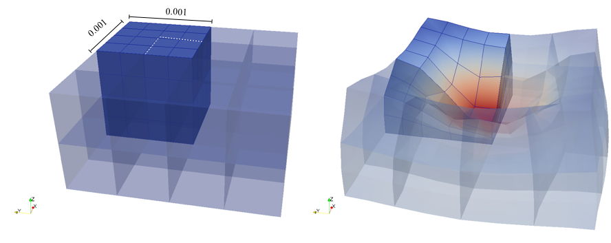
The material is quasi-incompressible neo-Hookean with shear modulus \(\mu = 80.194e6\) and \(\nu = 0.4999\). For such a choice of material properties a conventional single-field \(Q_1\) approach would lock. That is, the response would be overly stiff. The initial and final configurations are shown in the image above. Using symmetry, we solve for only one quarter of the geometry (i.e. a cube with dimension \(0.001\)). The inner-quarter of the upper surface of the domain is subject to a load of \(p_0\).
We start by including all the necessary deal.II header files and some C++ related ones. They have been discussed in detail in previous tutorial programs, so you need only refer to past tutorials for details.
This header gives us the functionality to store data at quadrature points
Here are the headers necessary to use the LinearOperator class. These are also all conveniently packaged into a single header file, namely <deal.II/lac/linear_operator_tools.h> but we list those specifically required here for the sake of transparency.
Defined in these two headers are some operations that are pertinent to finite strain elasticity. The first will help us compute some kinematic quantities, and the second provides some stanard tensor definitions.
We then stick everything that relates to this tutorial program into a namespace of its own, and import all the deal.II function and class names into it:
There are several parameters that can be set in the code so we set up a ParameterHandler object to read in the choices at run-time.
As mentioned in the introduction, a different order interpolation should be used for the displacement \(\mathbf{u}\) than for the pressure \(\widetilde{p}\) and the dilatation \(\widetilde{J}\). Choosing \(\widetilde{p}\) and \(\widetilde{J}\) as discontinuous (constant) functions at the element level leads to the mean-dilatation method. The discontinuous approximation allows \(\widetilde{p}\) and \(\widetilde{J}\) to be condensed out and a classical displacement based method is recovered. Here we specify the polynomial order used to approximate the solution. The quadrature order should be adjusted accordingly.
Make adjustments to the problem geometry and the applied load. Since the problem modelled here is quite specific, the load scale can be altered to specific values to compare with the results given in the literature.
We also need the shear modulus \( \mu \) and Poisson ration \( \nu \) for the neo-Hookean material.
Next, we choose both solver and preconditioner settings. The use of an effective preconditioner is critical to ensure convergence when a large nonlinear motion occurs within a Newton increment.
A Newton-Raphson scheme is used to solve the nonlinear system of governing equations. We now define the tolerances and the maximum number of iterations for the Newton-Raphson nonlinear solver.
Set the timestep size \( \varDelta t \) and the simulation end-time.
Finally we consolidate all of the above structures into a single container that holds all of our run-time selections.
A simple class to store time data. Its functioning is transparent so no discussion is necessary. For simplicity we assume a constant time step size.
As discussed in the Introduction, Neo-Hookean materials are a type of hyperelastic materials. The entire domain is assumed to be composed of a compressible neo-Hookean material. This class defines the behaviour of this material within a three-field formulation. Compressible neo-Hookean materials can be described by a strain-energy function (SEF) \( \Psi = \Psi_{\text{iso}}(\overline{\mathbf{b}}) + \Psi_{\text{vol}}(\widetilde{J}) \).
The isochoric response is given by \( \Psi_{\text{iso}}(\overline{\mathbf{b}}) = c_{1} [\overline{I}_{1} - 3] \) where \( c_{1} = \frac{\mu}{2} \) and \(\overline{I}_{1}\) is the first invariant of the left- or right-isochoric Cauchy-Green deformation tensors. That is \(\overline{I}_1 \dealcoloneq \textrm{tr}(\overline{\mathbf{b}})\). In this example the SEF that governs the volumetric response is defined as \( \Psi_{\text{vol}}(\widetilde{J}) = \kappa \frac{1}{4} [ \widetilde{J}^2 - 1 - 2\textrm{ln}\; \widetilde{J} ]\), where \(\kappa \dealcoloneq \lambda + 2/3 \mu\) is the bulk modulus and \(\lambda\) is Lame's first parameter.
The following class will be used to characterize the material we work with, and provides a central point that one would need to modify if one were to implement a different material model. For it to work, we will store one object of this type per quadrature point, and in each of these objects store the current state (characterized by the values or measures of the three fields) so that we can compute the elastic coefficients linearized around the current state.
We update the material model with various deformation dependent data based on \(F\) and the pressure \(\widetilde{p}\) and dilatation \(\widetilde{J}\), and at the end of the function include a physical check for internal consistency:
The second function determines the Kirchhoff stress \(\boldsymbol{\tau} = \boldsymbol{\tau}_{\textrm{iso}} + \boldsymbol{\tau}_{\textrm{vol}}\)
The fourth-order elasticity tensor in the spatial setting \(\mathfrak{c}\) is calculated from the SEF \(\Psi\) as \( J \mathfrak{c}_{ijkl} = F_{iA} F_{jB} \mathfrak{C}_{ABCD} F_{kC} F_{lD}\) where \( \mathfrak{C} = 4 \frac{\partial^2 \Psi(\mathbf{C})}{\partial \mathbf{C} \partial \mathbf{C}}\)
Derivative of the volumetric free energy with respect to \(\widetilde{J}\) return \(\frac{\partial \Psi_{\text{vol}}(\widetilde{J})}{\partial \widetilde{J}}\)
Second derivative of the volumetric free energy wrt \(\widetilde{J}\). We need the following computation explicitly in the tangent so we make it public. We calculate \(\frac{\partial^2 \Psi_{\textrm{vol}}(\widetilde{J})}{\partial \widetilde{J} \partial \widetilde{J}}\)
The next few functions return various data that we choose to store with the material:
Define constitutive model parameters \(\kappa\) (bulk modulus) and the neo-Hookean model parameter \(c_1\):
Model specific data that is convenient to store with the material:
The following functions are used internally in determining the result of some of the public functions above. The first one determines the volumetric Kirchhoff stress \(\boldsymbol{\tau}_{\textrm{vol}}\):
Next, determine the isochoric Kirchhoff stress \(\boldsymbol{\tau}_{\textrm{iso}} = \mathcal{P}:\overline{\boldsymbol{\tau}}\):
Then, determine the fictitious Kirchhoff stress \(\overline{\boldsymbol{\tau}}\):
Calculate the volumetric part of the tangent \(J \mathfrak{c}_\textrm{vol}\):
Calculate the isochoric part of the tangent \(J \mathfrak{c}_\textrm{iso}\):
Calculate the fictitious elasticity tensor \(\overline{\mathfrak{c}}\). For the material model chosen this is simply zero:
As seen in step-18, the PointHistory class offers a method for storing data at the quadrature points. Here each quadrature point holds a pointer to a material description. Thus, different material models can be used in different regions of the domain. Among other data, we choose to store the Kirchhoff stress \(\boldsymbol{\tau}\) and the tangent \(J\mathfrak{c}\) for the quadrature points.
The first function is used to create a material object and to initialize all tensors correctly: The second one updates the stored values and stresses based on the current deformation measure \(\textrm{Grad}\mathbf{u}_{\textrm{n}}\), pressure \(\widetilde{p}\) and dilation \(\widetilde{J}\) field values.
To this end, we calculate the deformation gradient \(\mathbf{F}\) from the displacement gradient \(\textrm{Grad}\ \mathbf{u}\), i.e. \(\mathbf{F}(\mathbf{u}) = \mathbf{I} + \textrm{Grad}\ \mathbf{u}\) and then let the material model associated with this quadrature point update itself. When computing the deformation gradient, we have to take care with which data types we compare the sum \(\mathbf{I} + \textrm{Grad}\ \mathbf{u}\): Since \(I\) has data type SymmetricTensor, just writing I + Grad_u_n would convert the second argument to a symmetric tensor, perform the sum, and then cast the result to a Tensor (i.e., the type of a possibly nonsymmetric tensor). However, since Grad_u_n is nonsymmetric in general, the conversion to SymmetricTensor will fail. We can avoid this back and forth by converting \(I\) to Tensor first, and then performing the addition as between nonsymmetric tensors:
The material has been updated so we now calculate the Kirchhoff stress \(\mathbf{\tau}\), the tangent \(J\mathfrak{c}\) and the first and second derivatives of the volumetric free energy.
We also store the inverse of the deformation gradient since we frequently use it:
We offer an interface to retrieve certain data. Here are the kinematic variables:
...and the kinetic variables. These are used in the material and global tangent matrix and residual assembly operations:
And finally the tangent:
In terms of member functions, this class stores for the quadrature point it represents a copy of a material type in case different materials are used in different regions of the domain, as well as the inverse of the deformation gradient...
... and stress-type variables along with the tangent \(J\mathfrak{c}\):
The Solid class is the central class in that it represents the problem at hand. It follows the usual scheme in that all it really has is a constructor, destructor and a run() function that dispatches all the work to private functions of this class:
In the private section of this class, we first forward declare a number of objects that are used in parallelizing work using the WorkStream object (see the Parallel computing with multiple processors accessing shared memory module for more information on this).
We declare such structures for the computation of tangent (stiffness) matrix, right hand side, static condensation, and for updating quadrature points:
We start the collection of member functions with one that builds the grid:
Set up the finite element system to be solved:
Several functions to assemble the system and right hand side matrices using multithreading. Each of them comes as a wrapper function, one that is executed to do the work in the WorkStream model on one cell, and one that copies the work done on this one cell into the global object that represents it:
Apply Dirichlet boundary conditions on the displacement field
Create and update the quadrature points. Here, no data needs to be copied into a global object, so the copy_local_to_global function is empty:
Solve for the displacement using a Newton-Raphson method. We break this function into the nonlinear loop and the function that solves the linearized Newton-Raphson step:
Solution retrieval as well as post-processing and writing data to file :
Finally, some member variables that describe the current state: A collection of the parameters used to describe the problem setup...
...the volume of the reference configuration...
...and description of the geometry on which the problem is solved:
Also, keep track of the current time and the time spent evaluating certain functions
A storage object for quadrature point information. As opposed to step-18, deal.II's native quadrature point data manager is employed here.
A description of the finite-element system including the displacement polynomial degree, the degree-of-freedom handler, number of DoFs per cell and the extractor objects used to retrieve information from the solution vectors:
Description of how the block-system is arranged. There are 3 blocks, the first contains a vector DOF \(\mathbf{u}\) while the other two describe scalar DOFs, \(\widetilde{p}\) and \(\widetilde{J}\).
Rules for Gauss-quadrature on both the cell and faces. The number of quadrature points on both cells and faces is recorded.
Objects that store the converged solution and right-hand side vectors, as well as the tangent matrix. There is an AffineConstraints object used to keep track of constraints. We make use of a sparsity pattern designed for a block system.
Then define a number of variables to store norms and update norms and normalization factors.
Methods to calculate error measures
Compute the volume in the spatial configuration
Print information to screen in a pleasing way...
Solid classWe initialize the Solid class using data extracted from the parameter file.
The Finite Element System is composed of dim continuous displacement DOFs, and discontinuous pressure and dilatation DOFs. In an attempt to satisfy the Babuska-Brezzi or LBB stability conditions (see Hughes (2000)), we setup a \(Q_n \times DGPM_{n-1} \times DGPM_{n-1}\) system. \(Q_2 \times DGPM_1 \times DGPM_1\) elements satisfy this condition, while \(Q_1 \times DGPM_0 \times DGPM_0\) elements do not. However, it has been shown that the latter demonstrate good convergence characteristics nonetheless.
In solving the quasi-static problem, the time becomes a loading parameter, i.e. we increasing the loading linearly with time, making the two concepts interchangeable. We choose to increment time linearly using a constant time step size.
We start the function with preprocessing, setting the initial dilatation values, and then output the initial grid before starting the simulation proper with the first time (and loading) increment.
Care must be taken (or at least some thought given) when imposing the constraint \(\widetilde{J}=1\) on the initial solution field. The constraint corresponds to the determinant of the deformation gradient in the undeformed configuration, which is the identity tensor. We use FE_DGPMonomial bases to interpolate the dilatation field, thus we can't simply set the corresponding dof to unity as they correspond to the monomial coefficients. Thus we use the VectorTools::project function to do the work for us. The VectorTools::project function requires an argument indicating the hanging node constraints. We have none in this program So we have to create a constraint object. In its original state, constraint objects are unsorted, and have to be sorted (using the AffineConstraints::close function) before they can be used. Have a look at step-21 for more information. We only need to enforce the initial condition on the dilatation. In order to do this, we make use of a ComponentSelectFunction which acts as a mask and sets the J_component of n_components to 1. This is exactly what we want. Have a look at its usage in step-20 for more information.
We then declare the incremental solution update \(\varDelta \mathbf{\Xi} \dealcoloneq \{\varDelta \mathbf{u},\varDelta \widetilde{p}, \varDelta \widetilde{J} \}\) and start the loop over the time domain.
At the beginning, we reset the solution update for this time step...
...solve the current time step and update total solution vector \(\mathbf{\Xi}_{\textrm{n}} = \mathbf{\Xi}_{\textrm{n-1}} + \varDelta \mathbf{\Xi}\)...
...and plot the results before moving on happily to the next time step:
The first group of private member functions is related to parallelization. We use the Threading Building Blocks library (TBB) to perform as many computationally intensive distributed tasks as possible. In particular, we assemble the tangent matrix and right hand side vector, the static condensation contributions, and update data stored at the quadrature points using TBB. Our main tool for this is the WorkStream class (see the Parallel computing with multiple processors accessing shared memory module for more information).
Firstly we deal with the tangent matrix assembly structures. The PerTaskData object stores local contributions.
On the other hand, the ScratchData object stores the larger objects such as the shape-function values array (Nx) and a shape function gradient and symmetric gradient vector which we will use during the assembly.
Next, the same approach is used for the right-hand side assembly. The PerTaskData object again stores local contributions and the ScratchData object the shape function object and precomputed values vector:
Then we define structures to assemble the statically condensed tangent matrix. Recall that we wish to solve for a displacement-based formulation. We do the condensation at the element level as the \(\widetilde{p}\) and \(\widetilde{J}\) fields are element-wise discontinuous. As these operations are matrix-based, we need to setup a number of matrices to store the local contributions from a number of the tangent matrix sub-blocks. We place these in the PerTaskData struct.
We choose not to reset any data in the reset() function as the matrix extraction and replacement tools will take care of this
The ScratchData object for the operations we wish to perform here is empty since we need no temporary data, but it still needs to be defined for the current implementation of TBB in deal.II. So we create a dummy struct for this purpose.
And finally we define the structures to assist with updating the quadrature point information. Similar to the SC assembly process, we do not need the PerTaskData object (since there is nothing to store here) but must define one nonetheless. Note that this is because for the operation that we have here – updating the data on quadrature points – the operation is purely local: the things we do on every cell get consumed on every cell, without any global aggregation operation as is usually the case when using the WorkStream class. The fact that we still have to define a per-task data structure points to the fact that the WorkStream class may be ill-suited to this operation (we could, in principle simply create a new task using Threads::new_task for each cell) but there is not much harm done to doing it this way anyway. Furthermore, should there be different material models associated with a quadrature point, requiring varying levels of computational expense, then the method used here could be advantageous.
The ScratchData object will be used to store an alias for the solution vector so that we don't have to copy this large data structure. We then define a number of vectors to extract the solution values and gradients at the quadrature points.
On to the first of the private member functions. Here we create the triangulation of the domain, for which we choose the scaled cube with each face given a boundary ID number. The grid must be refined at least once for the indentation problem.
We then determine the volume of the reference configuration and print it for comparison:
Since we wish to apply a Neumann BC to a patch on the top surface, we must find the cell faces in this part of the domain and mark them with a distinct boundary ID number. The faces we are looking for are on the +y surface and will get boundary ID 6 (zero through five are already used when creating the six faces of the cube domain):
Next we describe how the FE system is setup. We first determine the number of components per block. Since the displacement is a vector component, the first dim components belong to it, while the next two describe scalar pressure and dilatation DOFs.
The DOF handler is then initialized and we renumber the grid in an efficient manner. We also record the number of DOFs per block.
Setup the sparsity pattern and tangent matrix
The global system matrix initially has the following structure
\begin{align*} \underbrace{\begin{bmatrix} \mathsf{\mathbf{K}}_{uu} & \mathsf{\mathbf{K}}_{u\widetilde{p}} & \mathbf{0} \\ \mathsf{\mathbf{K}}_{\widetilde{p}u} & \mathbf{0} & \mathsf{\mathbf{K}}_{\widetilde{p}\widetilde{J}} \\ \mathbf{0} & \mathsf{\mathbf{K}}_{\widetilde{J}\widetilde{p}} & \mathsf{\mathbf{K}}_{\widetilde{J}\widetilde{J}} \end{bmatrix}}_{\mathsf{\mathbf{K}}(\mathbf{\Xi}_{\textrm{i}})} \underbrace{\begin{bmatrix} d \mathsf{u} \\ d \widetilde{\mathsf{\mathbf{p}}} \\ d \widetilde{\mathsf{\mathbf{J}}} \end{bmatrix}}_{d \mathbf{\Xi}} = \underbrace{\begin{bmatrix} \mathsf{\mathbf{F}}_{u}(\mathbf{u}_{\textrm{i}}) \\ \mathsf{\mathbf{F}}_{\widetilde{p}}(\widetilde{p}_{\textrm{i}}) \\ \mathsf{\mathbf{F}}_{\widetilde{J}}(\widetilde{J}_{\textrm{i}}) \end{bmatrix}}_{ \mathsf{\mathbf{F}}(\mathbf{\Xi}_{\textrm{i}}) } \, . \end{align*}
We optimize the sparsity pattern to reflect this structure and prevent unnecessary data creation for the right-diagonal block components.
We then set up storage vectors
...and finally set up the quadrature point history:
Next we compute some information from the FE system that describes which local element DOFs are attached to which block component. This is used later to extract sub-blocks from the global matrix.
In essence, all we need is for the FESystem object to indicate to which block component a DOF on the reference cell is attached to. Currently, the interpolation fields are setup such that 0 indicates a displacement DOF, 1 a pressure DOF and 2 a dilatation DOF.
The method used to store quadrature information is already described in step-18. Here we implement a similar setup for a SMP machine.
Firstly the actual QPH data objects are created. This must be done only once the grid is refined to its finest level.
Next we setup the initial quadrature point data. Note that when the quadrature point data is retrieved, it is returned as a vector of smart pointers.
As the update of QP information occurs frequently and involves a number of expensive operations, we define a multithreaded approach to distributing the task across a number of CPU cores.
To start this, we first we need to obtain the total solution as it stands at this Newton increment and then create the initial copy of the scratch and copy data objects:
We then pass them and the one-cell update function to the WorkStream to be processed:
Now we describe how we extract data from the solution vector and pass it along to each QP storage object for processing.
We first need to find the values and gradients at quadrature points inside the current cell and then we update each local QP using the displacement gradient and total pressure and dilatation solution values:
The next function is the driver method for the Newton-Raphson scheme. At its top we create a new vector to store the current Newton update step, reset the error storage objects and print solver header.
We now perform a number of Newton iterations to iteratively solve the nonlinear problem. Since the problem is fully nonlinear and we are using a full Newton method, the data stored in the tangent matrix and right-hand side vector is not reusable and must be cleared at each Newton step. We then initially build the right-hand side vector to check for convergence (and store this value in the first iteration). The unconstrained DOFs of the rhs vector hold the out-of-balance forces. The building is done before assembling the system matrix as the latter is an expensive operation and we can potentially avoid an extra assembly process by not assembling the tangent matrix when convergence is attained.
We can now determine the normalized residual error and check for solution convergence:
If we have decided that we want to continue with the iteration, we assemble the tangent, make and impose the Dirichlet constraints, and do the solve of the linearised system:
We can now determine the normalized Newton update error, and perform the actual update of the solution increment for the current time step, update all quadrature point information pertaining to this new displacement and stress state and continue iterating:
At the end, if it turns out that we have in fact done more iterations than the parameter file allowed, we raise an exception that can be caught in the main() function. The call AssertThrow(condition, exc_object) is in essence equivalent to if (!cond) throw exc_object; but the former form fills certain fields in the exception object that identify the location (filename and line number) where the exception was raised to make it simpler to identify where the problem happened.
This program prints out data in a nice table that is updated on a per-iteration basis. The next two functions set up the table header and footer:
Calculate the volume of the domain in the spatial configuration
In contrast to that which was previously called for, in this instance the quadrature point data is specifically non-modifiable since we will only be accessing data. We ensure that the right get_data function is called by marking this update function as constant.
Calculate how well the dilatation \(\widetilde{J}\) agrees with \(J \dealcoloneq \textrm{det}\ \mathbf{F}\) from the \(L^2\) error \( \bigl[ \int_{\Omega_0} {[ J - \widetilde{J}]}^{2}\textrm{d}V \bigr]^{1/2}\). We also return the ratio of the current volume of the domain to the reference volume. This is of interest for incompressible media where we want to check how well the isochoric constraint has been enforced.
Determine the true residual error for the problem. That is, determine the error in the residual for the unconstrained degrees of freedom. Note that to do so, we need to ignore constrained DOFs by setting the residual in these vector components to zero.
Determine the true Newton update error for the problem
This function provides the total solution, which is valid at any Newton step. This is required as, to reduce computational error, the total solution is only updated at the end of the timestep.
Since we use TBB for assembly, we simply setup a copy of the data structures required for the process and pass them, along with the memory addresses of the assembly functions to the WorkStream object for processing. Note that we must ensure that the matrix is reset before any assembly operations can occur.
The syntax used here to pass data to the WorkStream class is discussed in step-14. We need to use this particular call to WorkStream because assemble_system_tangent_one_cell is a constant function and copy_local_to_global_K is non-constant.
This function adds the local contribution to the system matrix. Note that we choose not to use the constraint matrix to do the job for us because the tangent matrix and residual processes have been split up into two separate functions.
Of course, we still have to define how we assemble the tangent matrix contribution for a single cell. We first need to reset and initialize some of the scratch data structures and retrieve some basic information regarding the DOF numbering on this cell. We can precalculate the cell shape function values and gradients. Note that the shape function gradients are defined with regard to the current configuration. That is \(\textrm{grad}\ \boldsymbol{\varphi} = \textrm{Grad}\ \boldsymbol{\varphi} \ \mathbf{F}^{-1}\).
Now we build the local cell stiffness matrix. Since the global and local system matrices are symmetric, we can exploit this property by building only the lower half of the local matrix and copying the values to the upper half. So we only assemble half of the \(\mathsf{\mathbf{k}}_{uu}\), \(\mathsf{\mathbf{k}}_{\widetilde{p} \widetilde{p}} = \mathbf{0}\), \(\mathsf{\mathbf{k}}_{\widetilde{J} \widetilde{J}}\) blocks, while the whole \(\mathsf{\mathbf{k}}_{\widetilde{p} \widetilde{J}}\), \(\mathsf{\mathbf{k}}_{u \widetilde{J}} = \mathbf{0}\), \(\mathsf{\mathbf{k}}_{u \widetilde{p}}\) blocks are built.
In doing so, we first extract some configuration dependent variables from our quadrature history objects for the current quadrature point.
Next we define some aliases to make the assembly process easier to follow
This is the \(\mathsf{\mathbf{k}}_{uu}\) contribution. It comprises a material contribution, and a geometrical stress contribution which is only added along the local matrix diagonals:
The material contribution:
The geometrical stress contribution:
Next is the \(\mathsf{\mathbf{k}}_{ \widetilde{p} u}\) contribution
and lastly the \(\mathsf{\mathbf{k}}_{ \widetilde{J} \widetilde{p}}\) and \(\mathsf{\mathbf{k}}_{ \widetilde{J} \widetilde{J}}\) contributions:
Finally, we need to copy the lower half of the local matrix into the upper half:
The assembly of the right-hand side process is similar to the tangent matrix, so we will not describe it in too much detail. Note that since we are describing a problem with Neumann BCs, we will need the face normals and so must specify this in the update flags.
We first compute the contributions from the internal forces. Note, by definition of the rhs as the negative of the residual, these contributions are subtracted.
Next we assemble the Neumann contribution. We first check to see it the cell face exists on a boundary on which a traction is applied and add the contribution if this is the case.
Using the face normal at this quadrature point we specify the traction in reference configuration. For this problem, a defined pressure is applied in the reference configuration. The direction of the applied traction is assumed not to evolve with the deformation of the domain. The traction is defined using the first Piola-Kirchhoff stress is simply \(\mathbf{t} = \mathbf{P}\mathbf{N} = [p_0 \mathbf{I}] \mathbf{N} = p_0 \mathbf{N}\) We use the time variable to linearly ramp up the pressure load.
Note that the contributions to the right hand side vector we compute here only exist in the displacement components of the vector.
The constraints for this problem are simple to describe. However, since we are dealing with an iterative Newton method, it should be noted that any displacement constraints should only be specified at the zeroth iteration and subsequently no additional contributions are to be made since the constraints are already exactly satisfied.
Since the constraints are different at different Newton iterations, we need to clear the constraints matrix and completely rebuild it. However, after the first iteration, the constraints remain the same and we can simply skip the rebuilding step if we do not clear it.
In this particular example, the boundary values will be calculated for the two first iterations of Newton's algorithm. In general, one would build non-homogeneous constraints in the zeroth iteration (that is, when apply_dirichlet_bc == true) and build only the corresponding homogeneous constraints in the following step. While the current example has only homogeneous constraints, previous experiences have shown that a common error is forgetting to add the extra condition when refactoring the code to specific uses. This could lead errors that are hard to debug. In this spirit, we choose to make the code more verbose in terms of what operations are performed at each Newton step.
The boundary conditions for the indentation problem are as follows: On the -x, -y and -z faces (IDs 0,2,4) we set up a symmetry condition to allow only planar movement while the +x and +z faces (IDs 1,5) are traction free. In this contrived problem, part of the +y face (ID 3) is set to have no motion in the x- and z-component. Finally, as described earlier, the other part of the +y face has an the applied pressure but is also constrained in the x- and z-directions.
In the following, we will have to tell the function interpolation boundary values which components of the solution vector should be constrained (i.e., whether it's the x-, y-, z-displacements or combinations thereof). This is done using ComponentMask objects (see GlossComponentMask) which we can get from the finite element if we provide it with an extractor object for the component we wish to select. To this end we first set up such extractor objects and later use it when generating the relevant component masks:
Solving the entire block system is a bit problematic as there are no contributions to the \(\mathsf{\mathbf{K}}_{ \widetilde{J} \widetilde{J}}\) block, rendering it noninvertible (when using an iterative solver). Since the pressure and dilatation variables DOFs are discontinuous, we can condense them out to form a smaller displacement-only system which we will then solve and subsequently post-process to retrieve the pressure and dilatation solutions.
The static condensation process could be performed at a global level but we need the inverse of one of the blocks. However, since the pressure and dilatation variables are discontinuous, the static condensation (SC) operation can also be done on a per-cell basis and we can produce the inverse of the block-diagonal \(\mathsf{\mathbf{K}}_{\widetilde{p}\widetilde{J}}\) block by inverting the local blocks. We can again use TBB to do this since each operation will be independent of one another.
Using the TBB via the WorkStream class, we assemble the contributions to form \( \mathsf{\mathbf{K}}_{\textrm{con}} = \bigl[ \mathsf{\mathbf{K}}_{uu} + \overline{\overline{\mathsf{\mathbf{K}}}}~ \bigr] \) from each element's contributions. These contributions are then added to the global stiffness matrix. Given this description, the following two functions should be clear:
Now we describe the static condensation process. As per usual, we must first find out which global numbers the degrees of freedom on this cell have and reset some data structures:
We now extract the contribution of the dofs associated with the current cell to the global stiffness matrix. The discontinuous nature of the \(\widetilde{p}\) and \(\widetilde{J}\) interpolations mean that their is no coupling of the local contributions at the global level. This is not the case with the \(\mathbf{u}\) dof. In other words, \(\mathsf{\mathbf{k}}_{\widetilde{J} \widetilde{p}}\), \(\mathsf{\mathbf{k}}_{\widetilde{p} \widetilde{p}}\) and \(\mathsf{\mathbf{k}}_{\widetilde{J} \widetilde{p}}\), when extracted from the global stiffness matrix are the element contributions. This is not the case for \(\mathsf{\mathbf{k}}_{uu}\).
Note: A lower-case symbol is used to denote element stiffness matrices.
Currently the matrix corresponding to the dof associated with the current element (denoted somewhat loosely as \(\mathsf{\mathbf{k}}\)) is of the form:
\begin{align*} \begin{bmatrix} \mathsf{\mathbf{k}}_{uu} & \mathsf{\mathbf{k}}_{u\widetilde{p}} & \mathbf{0} \\ \mathsf{\mathbf{k}}_{\widetilde{p}u} & \mathbf{0} & \mathsf{\mathbf{k}}_{\widetilde{p}\widetilde{J}} \\ \mathbf{0} & \mathsf{\mathbf{k}}_{\widetilde{J}\widetilde{p}} & \mathsf{\mathbf{k}}_{\widetilde{J}\widetilde{J}} \end{bmatrix} \end{align*}
We now need to modify it such that it appear as
\begin{align*} \begin{bmatrix} \mathsf{\mathbf{k}}_{\textrm{con}} & \mathsf{\mathbf{k}}_{u\widetilde{p}} & \mathbf{0} \\ \mathsf{\mathbf{k}}_{\widetilde{p}u} & \mathbf{0} & \mathsf{\mathbf{k}}_{\widetilde{p}\widetilde{J}}^{-1} \\ \mathbf{0} & \mathsf{\mathbf{k}}_{\widetilde{J}\widetilde{p}} & \mathsf{\mathbf{k}}_{\widetilde{J}\widetilde{J}} \end{bmatrix} \end{align*}
with \(\mathsf{\mathbf{k}}_{\textrm{con}} = \bigl[ \mathsf{\mathbf{k}}_{uu} +\overline{\overline{\mathsf{\mathbf{k}}}}~ \bigr]\) where \( \overline{\overline{\mathsf{\mathbf{k}}}} \dealcoloneq \mathsf{\mathbf{k}}_{u\widetilde{p}} \overline{\mathsf{\mathbf{k}}} \mathsf{\mathbf{k}}_{\widetilde{p}u} \) and \( \overline{\mathsf{\mathbf{k}}} = \mathsf{\mathbf{k}}_{\widetilde{J}\widetilde{p}}^{-1} \mathsf{\mathbf{k}}_{\widetilde{J}\widetilde{J}} \mathsf{\mathbf{k}}_{\widetilde{p}\widetilde{J}}^{-1} \).
At this point, we need to take note of the fact that global data already exists in the \(\mathsf{\mathbf{K}}_{uu}\), \(\mathsf{\mathbf{K}}_{\widetilde{p} \widetilde{J}}\) and \(\mathsf{\mathbf{K}}_{\widetilde{J} \widetilde{p}}\) sub-blocks. So if we are to modify them, we must account for the data that is already there (i.e. simply add to it or remove it if necessary). Since the copy_local_to_global operation is a "+=" operation, we need to take this into account
For the \(\mathsf{\mathbf{K}}_{uu}\) block in particular, this means that contributions have been added from the surrounding cells, so we need to be careful when we manipulate this block. We can't just erase the sub-blocks.
This is the strategy we will employ to get the sub-blocks we want:
We first extract element data from the system matrix. So first we get the entire subblock for the cell, then extract \(\mathsf{\mathbf{k}}\) for the dofs associated with the current element
and next the local matrices for \(\mathsf{\mathbf{k}}_{ \widetilde{p} u}\) \(\mathsf{\mathbf{k}}_{ \widetilde{p} \widetilde{J}}\) and \(\mathsf{\mathbf{k}}_{ \widetilde{J} \widetilde{J}}\):
To get the inverse of \(\mathsf{\mathbf{k}}_{\widetilde{p} \widetilde{J}}\), we invert it directly. This operation is relatively inexpensive since \(\mathsf{\mathbf{k}}_{\widetilde{p} \widetilde{J}}\) since block-diagonal.
Now we can make condensation terms to add to the \(\mathsf{\mathbf{k}}_{uu}\) block and put them in the cell local matrix \( \mathsf{\mathbf{A}} = \mathsf{\mathbf{k}}^{-1}_{\widetilde{p} \widetilde{J}} \mathsf{\mathbf{k}}_{\widetilde{p} u} \):
\( \mathsf{\mathbf{B}} = \mathsf{\mathbf{k}}^{-1}_{\widetilde{J} \widetilde{J}} \mathsf{\mathbf{k}}^{-1}_{\widetilde{p} \widetilde{J}} \mathsf{\mathbf{k}}_{\widetilde{p} u} \)
\( \mathsf{\mathbf{C}} = \mathsf{\mathbf{k}}^{-1}_{\widetilde{J} \widetilde{p}} \mathsf{\mathbf{k}}^{-1}_{\widetilde{J} \widetilde{J}} \mathsf{\mathbf{k}}^{-1}_{\widetilde{p} \widetilde{J}} \mathsf{\mathbf{k}}_{\widetilde{p} u} \)
\( \overline{\overline{\mathsf{\mathbf{k}}}} = \mathsf{\mathbf{k}}_{u \widetilde{p}} \mathsf{\mathbf{k}}^{-1}_{\widetilde{J} \widetilde{p}} \mathsf{\mathbf{k}}^{-1}_{\widetilde{J} \widetilde{J}} \mathsf{\mathbf{k}}^{-1}_{\widetilde{p} \widetilde{J}} \mathsf{\mathbf{k}}_{\widetilde{p} u} \)
Next we place \(\mathsf{\mathbf{k}}^{-1}_{ \widetilde{p} \widetilde{J}}\) in the \(\mathsf{\mathbf{k}}_{ \widetilde{p} \widetilde{J}}\) block for post-processing. Note again that we need to remove the contribution that already exists there.
We now have all of the necessary components to use one of two possible methods to solve the linearised system. The first is to perform static condensation on an element level, which requires some alterations to the tangent matrix and RHS vector. Alternatively, the full block system can be solved by performing condensation on a global level. Below we implement both approaches.
Firstly, here is the approach using the (permanent) augmentation of the tangent matrix. For the following, recall that
\begin{align*} \mathsf{\mathbf{K}}_{\textrm{store}} \dealcoloneq \begin{bmatrix} \mathsf{\mathbf{K}}_{\textrm{con}} & \mathsf{\mathbf{K}}_{u\widetilde{p}} & \mathbf{0} \\ \mathsf{\mathbf{K}}_{\widetilde{p}u} & \mathbf{0} & \mathsf{\mathbf{K}}_{\widetilde{p}\widetilde{J}}^{-1} \\ \mathbf{0} & \mathsf{\mathbf{K}}_{\widetilde{J}\widetilde{p}} & \mathsf{\mathbf{K}}_{\widetilde{J}\widetilde{J}} \end{bmatrix} \, . \end{align*}
and
\begin{align*} d \widetilde{\mathsf{\mathbf{p}}} & = \mathsf{\mathbf{K}}_{\widetilde{J}\widetilde{p}}^{-1} \bigl[ \mathsf{\mathbf{F}}_{\widetilde{J}} - \mathsf{\mathbf{K}}_{\widetilde{J}\widetilde{J}} d \widetilde{\mathsf{\mathbf{J}}} \bigr] \\ d \widetilde{\mathsf{\mathbf{J}}} & = \mathsf{\mathbf{K}}_{\widetilde{p}\widetilde{J}}^{-1} \bigl[ \mathsf{\mathbf{F}}_{\widetilde{p}} - \mathsf{\mathbf{K}}_{\widetilde{p}u} d \mathsf{\mathbf{u}} \bigr] \\ \Rightarrow d \widetilde{\mathsf{\mathbf{p}}} &= \mathsf{\mathbf{K}}_{\widetilde{J}\widetilde{p}}^{-1} \mathsf{\mathbf{F}}_{\widetilde{J}} - \underbrace{\bigl[\mathsf{\mathbf{K}}_{\widetilde{J}\widetilde{p}}^{-1} \mathsf{\mathbf{K}}_{\widetilde{J}\widetilde{J}} \mathsf{\mathbf{K}}_{\widetilde{p}\widetilde{J}}^{-1}\bigr]}_{\overline{\mathsf{\mathbf{K}}}}\bigl[ \mathsf{\mathbf{F}}_{\widetilde{p}} - \mathsf{\mathbf{K}}_{\widetilde{p}u} d \mathsf{\mathbf{u}} \bigr] \end{align*}
and thus
\[ \underbrace{\bigl[ \mathsf{\mathbf{K}}_{uu} + \overline{\overline{\mathsf{\mathbf{K}}}}~ \bigr] }_{\mathsf{\mathbf{K}}_{\textrm{con}}} d \mathsf{\mathbf{u}} = \underbrace{ \Bigl[ \mathsf{\mathbf{F}}_{u} - \mathsf{\mathbf{K}}_{u\widetilde{p}} \bigl[ \mathsf{\mathbf{K}}_{\widetilde{J}\widetilde{p}}^{-1} \mathsf{\mathbf{F}}_{\widetilde{J}} - \overline{\mathsf{\mathbf{K}}}\mathsf{\mathbf{F}}_{\widetilde{p}} \bigr] \Bigr]}_{\mathsf{\mathbf{F}}_{\textrm{con}}} \]
where
\[ \overline{\overline{\mathsf{\mathbf{K}}}} \dealcoloneq \mathsf{\mathbf{K}}_{u\widetilde{p}} \overline{\mathsf{\mathbf{K}}} \mathsf{\mathbf{K}}_{\widetilde{p}u} \, . \]
At the top, we allocate two temporary vectors to help with the static condensation, and variables to store the number of linear solver iterations and the (hopefully converged) residual.
In the first step of this function, we solve for the incremental displacement \(d\mathbf{u}\). To this end, we perform static condensation to make \(\mathsf{\mathbf{K}}_{\textrm{con}} = \bigl[ \mathsf{\mathbf{K}}_{uu} + \overline{\overline{\mathsf{\mathbf{K}}}}~ \bigr]\) and put \(\mathsf{\mathbf{K}}^{-1}_{\widetilde{p} \widetilde{J}}\) in the original \(\mathsf{\mathbf{K}}_{\widetilde{p} \widetilde{J}}\) block. That is, we make \(\mathsf{\mathbf{K}}_{\textrm{store}}\).
\( \mathsf{\mathbf{A}}_{\widetilde{J}} = \mathsf{\mathbf{K}}^{-1}_{\widetilde{p} \widetilde{J}} \mathsf{\mathbf{F}}_{\widetilde{p}} \)
\( \mathsf{\mathbf{B}}_{\widetilde{J}} = \mathsf{\mathbf{K}}_{\widetilde{J} \widetilde{J}} \mathsf{\mathbf{K}}^{-1}_{\widetilde{p} \widetilde{J}} \mathsf{\mathbf{F}}_{\widetilde{p}} \)
\( \mathsf{\mathbf{A}}_{\widetilde{J}} = \mathsf{\mathbf{F}}_{\widetilde{J}} - \mathsf{\mathbf{K}}_{\widetilde{J} \widetilde{J}} \mathsf{\mathbf{K}}^{-1}_{\widetilde{p} \widetilde{J}} \mathsf{\mathbf{F}}_{\widetilde{p}} \)
\( \mathsf{\mathbf{A}}_{\widetilde{J}} = \mathsf{\mathbf{K}}^{-1}_{\widetilde{J} \widetilde{p}} [ \mathsf{\mathbf{F}}_{\widetilde{J}} - \mathsf{\mathbf{K}}_{\widetilde{J} \widetilde{J}} \mathsf{\mathbf{K}}^{-1}_{\widetilde{p} \widetilde{J}} \mathsf{\mathbf{F}}_{\widetilde{p}} ] \)
\( \mathsf{\mathbf{A}}_{u} = \mathsf{\mathbf{K}}_{u \widetilde{p}} \mathsf{\mathbf{K}}^{-1}_{\widetilde{J} \widetilde{p}} [ \mathsf{\mathbf{F}}_{\widetilde{J}} - \mathsf{\mathbf{K}}_{\widetilde{J} \widetilde{J}} \mathsf{\mathbf{K}}^{-1}_{\widetilde{p} \widetilde{J}} \mathsf{\mathbf{F}}_{\widetilde{p}} ] \)
\( \mathsf{\mathbf{F}}_{\text{con}} = \mathsf{\mathbf{F}}_{u} - \mathsf{\mathbf{K}}_{u \widetilde{p}} \mathsf{\mathbf{K}}^{-1}_{\widetilde{J} \widetilde{p}} [ \mathsf{\mathbf{F}}_{\widetilde{J}} - \mathsf{\mathbf{K}}_{\widetilde{J} \widetilde{J}} \mathsf{\mathbf{K}}^{-1}_{\widetilde{p} \widetilde{J}} \mathsf{\mathbf{F}}_{\widetilde{p}} ] \)
We've chosen by default a SSOR preconditioner as it appears to provide the fastest solver convergence characteristics for this problem on a single-thread machine. However, this might not be true for different problem sizes.
Otherwise if the problem is small enough, a direct solver can be utilised.
Now that we have the displacement update, distribute the constraints back to the Newton update:
The next step after solving the displacement problem is to post-process to get the dilatation solution from the substitution: \( d \widetilde{\mathsf{\mathbf{J}}} = \mathsf{\mathbf{K}}_{\widetilde{p}\widetilde{J}}^{-1} \bigl[ \mathsf{\mathbf{F}}_{\widetilde{p}} - \mathsf{\mathbf{K}}_{\widetilde{p}u} d \mathsf{\mathbf{u}} \bigr] \)
\( \mathsf{\mathbf{A}}_{\widetilde{p}} = \mathsf{\mathbf{K}}_{\widetilde{p}u} d \mathsf{\mathbf{u}} \)
\( \mathsf{\mathbf{A}}_{\widetilde{p}} = -\mathsf{\mathbf{K}}_{\widetilde{p}u} d \mathsf{\mathbf{u}} \)
\( \mathsf{\mathbf{A}}_{\widetilde{p}} = \mathsf{\mathbf{F}}_{\widetilde{p}} -\mathsf{\mathbf{K}}_{\widetilde{p}u} d \mathsf{\mathbf{u}} \)
\( d\mathsf{\mathbf{\widetilde{J}}} = \mathsf{\mathbf{K}}^{-1}_{\widetilde{p}\widetilde{J}} [ \mathsf{\mathbf{F}}_{\widetilde{p}} -\mathsf{\mathbf{K}}_{\widetilde{p}u} d \mathsf{\mathbf{u}} ] \)
we ensure here that any Dirichlet constraints are distributed on the updated solution:
Finally we solve for the pressure update with the substitution: \( d \widetilde{\mathsf{\mathbf{p}}} = \mathsf{\mathbf{K}}_{\widetilde{J}\widetilde{p}}^{-1} \bigl[ \mathsf{\mathbf{F}}_{\widetilde{J}} - \mathsf{\mathbf{K}}_{\widetilde{J}\widetilde{J}} d \widetilde{\mathsf{\mathbf{J}}} \bigr] \)
\( \mathsf{\mathbf{A}}_{\widetilde{J}} = \mathsf{\mathbf{K}}_{\widetilde{J}\widetilde{J}} d \widetilde{\mathsf{\mathbf{J}}} \)
\( \mathsf{\mathbf{A}}_{\widetilde{J}} = -\mathsf{\mathbf{K}}_{\widetilde{J}\widetilde{J}} d \widetilde{\mathsf{\mathbf{J}}} \)
\( \mathsf{\mathbf{A}}_{\widetilde{J}} = \mathsf{\mathbf{F}}_{\widetilde{J}} - \mathsf{\mathbf{K}}_{\widetilde{J}\widetilde{J}} d \widetilde{\mathsf{\mathbf{J}}} \)
and finally.... \( d \widetilde{\mathsf{\mathbf{p}}} = \mathsf{\mathbf{K}}_{\widetilde{J}\widetilde{p}}^{-1} \bigl[ \mathsf{\mathbf{F}}_{\widetilde{J}} - \mathsf{\mathbf{K}}_{\widetilde{J}\widetilde{J}} d \widetilde{\mathsf{\mathbf{J}}} \bigr] \)
We are now at the end, so we distribute all constrained dofs back to the Newton update:
Manual condensation of the dilatation and pressure fields on a local level, and subsequent post-processing, took quite a bit of effort to achieve. To recap, we had to produce the inverse matrix \(\mathsf{\mathbf{K}}_{\widetilde{p}\widetilde{J}}^{-1}\), which was permanently written into the global tangent matrix. We then permanently modified \(\mathsf{\mathbf{K}}_{uu}\) to produce \(\mathsf{\mathbf{K}}_{\textrm{con}}\). This involved the extraction and manipulation of local sub-blocks of the tangent matrix. After solving for the displacement, the individual matrix-vector operations required to solve for dilatation and pressure were carefully implemented. Contrast these many sequence of steps to the much simpler and transparent implementation using functionality provided by the LinearOperator class.
For ease of later use, we define some aliases for blocks in the RHS vector
... and for blocks in the Newton update vector.
We next define some linear operators for the tangent matrix sub-blocks We will exploit the symmetry of the system, so not all blocks are required.
We then construct a LinearOperator that represents the inverse of (square block) \(\mathsf{\mathbf{K}}_{\widetilde{J}\widetilde{p}}\). Since it is diagonal (or, when a higher order ansatz it used, nearly diagonal), a Jacobi preconditioner is suitable.
Now we can construct that transpose of \(\mathsf{\mathbf{K}}_{\widetilde{J}\widetilde{p}}^{-1}\) and a linear operator that represents the condensed operations \(\overline{\mathsf{\mathbf{K}}}\) and \(\overline{\overline{\mathsf{\mathbf{K}}}}\) and the final augmented matrix \(\mathsf{\mathbf{K}}_{\textrm{con}}\). Note that the schur_complement() operator could also be of use here, but for clarity and the purpose of demonstrating the similarities between the formulation and implementation of the linear solution scheme, we will perform these operations manually.
Lastly, we define an operator for inverse of augmented stiffness matrix, namely \(\mathsf{\mathbf{K}}_{\textrm{con}}^{-1}\). Note that the preconditioner for the augmented stiffness matrix is different to the case when we use static condensation. In this instance, the preconditioner is based on a non-modified \(\mathsf{\mathbf{K}}_{uu}\), while with the first approach we actually modified the entries of this sub-block. However, since \(\mathsf{\mathbf{K}}_{\textrm{con}}\) and \(\mathsf{\mathbf{K}}_{uu}\) operate on the same space, it remains adequate for this problem.
Now we are in a position to solve for the displacement field. We can nest the linear operations, and the result is immediately written to the Newton update vector. It is clear that the implementation closely mimics the derivation stated in the introduction.
The operations need to post-process for the dilatation and pressure fields are just as easy to express.
Solve the full block system with a direct solver. As it is relatively robust, it may be immune to problem arising from the presence of the zero \(\mathsf{\mathbf{K}}_{ \widetilde{J} \widetilde{J}}\) block.
Finally, we again ensure here that any Dirichlet constraints are distributed on the updated solution:
Here we present how the results are written to file to be viewed using ParaView or Visit. The method is similar to that shown in previous tutorials so will not be discussed in detail.
Since we are dealing with a large deformation problem, it would be nice to display the result on a displaced grid! The MappingQEulerian class linked with the DataOut class provides an interface through which this can be achieved without physically moving the grid points in the Triangulation object ourselves. We first need to copy the solution to a temporary vector and then create the Eulerian mapping. We also specify the polynomial degree to the DataOut object in order to produce a more refined output data set when higher order polynomials are used.
Lastly we provide the main driver function which appears no different to the other tutorials.
Firstly, we present a comparison of a series of 3-d results with those in the literature (see Reese et al (2000)) to demonstrate that the program works as expected.
We begin with a comparison of the convergence with mesh refinement for the \(Q_1-DGPM_0-DGPM_0\) and \(Q_2-DGPM_1-DGPM_1\) formulations, as summarised in the figure below. The vertical displacement of the midpoint of the upper surface of the block is used to assess convergence. Both schemes demonstrate good convergence properties for varying values of the load parameter \(p/p_0\). The results agree with those in the literature. The lower-order formulation typically overestimates the displacement for low levels of refinement, while the higher-order interpolation scheme underestimates it, but be a lesser degree. This benchmark, and a series of others not shown here, give us confidence that the code is working as it should.
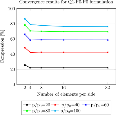
Convergence of the \(Q_1-DGPM_0-DGPM_0\) formulation in 3-d. | 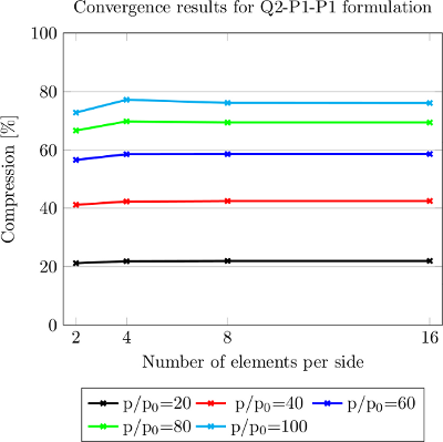
Convergence of the \(Q_2-DGPM_1-DGPM_1\) formulation in 3-d. |
A typical screen output generated by running the problem is shown below. The particular case demonstrated is that of the \(Q_2-DGPM_1-DGPM_1\) formulation. It is clear that, using the Newton-Raphson method, quadratic convergence of the solution is obtained. Solution convergence is achieved within 5 Newton increments for all time-steps. The converged displacement's \(L_2\)-norm is several orders of magnitude less than the geometry scale.
Using the Timer class, we can discern which parts of the code require the highest computational expense. For a case with a large number of degrees-of-freedom (i.e. a high level of refinement), a typical output of the Timer is given below. Much of the code in the tutorial has been developed based on the optimizations described, discussed and demonstrated in step-18 and others. With over 93% of the time being spent in the linear solver, it is obvious that it may be necessary to invest in a better solver for large three-dimensional problems. The SSOR preconditioner is not multithreaded but is effective for this class of solid problems. It may be beneficial to investigate the use of another solver such as those available through the Trilinos library.
We then used ParaView to visualize the results for two cases. The first was for the coarsest grid and the lowest-order interpolation method: \(Q_1-DGPM_0-DGPM_0\). The second was on a refined grid using a \(Q_2-DGPM_1-DGPM_1\) formulation. The vertical component of the displacement, the pressure \(\widetilde{p}\) and the dilatation \(\widetilde{J}\) fields are shown below.
For the first case it is clear that the coarse spatial discretization coupled with large displacements leads to a low quality solution (the loading ratio is \(p/p_0=80\)). Additionally, the pressure difference between elements is very large. The constant pressure field on the element means that the large pressure gradient is not captured. However, it should be noted that locking, which would be present in a standard \(Q_1\) displacement formulation does not arise even in this poorly discretised case. The final vertical displacement of the tracked node on the top surface of the block is still within 12.5% of the converged solution. The pressure solution is very coarse and has large jumps between adjacent cells. It is clear that the volume nearest to the applied traction undergoes compression while the outer extents of the domain are in a state of expansion. The dilatation solution field and pressure field are clearly linked, with positive dilatation indicating regions of positive pressure and negative showing regions placed in compression. As discussed in the Introduction, a compressive pressure has a negative sign while an expansive pressure takes a positive sign. This stems from the definition of the volumetric strain energy function and is opposite to the physically realistic interpretation of pressure.
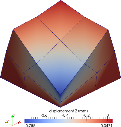
Z-displacement solution for the 3-d problem. | 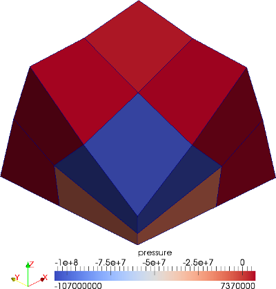
Discontinuous piece-wise constant pressure field. | 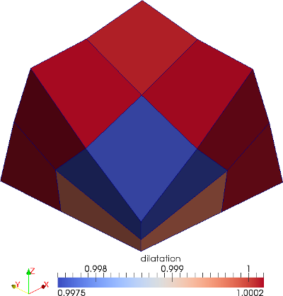
Discontinuous piece-wise constant dilatation field. |
Combining spatial refinement and a higher-order interpolation scheme results in a high-quality solution. Three grid refinements coupled with a \(Q_2-DGPM_1-DGPM_1\) formulation produces a result that clearly captures the mechanics of the problem. The deformation of the traction surface is well resolved. We can now observe the actual extent of the applied traction, with the maximum force being applied at the central point of the surface causing the largest compression. Even though very high strains are experienced in the domain, especially at the boundary of the region of applied traction, the solution remains accurate. The pressure field is captured in far greater detail than before. There is a clear distinction and transition between regions of compression and expansion, and the linear approximation of the pressure field allows a refined visualization of the pressure at the sub-element scale. It should however be noted that the pressure field remains discontinuous and could be smoothed on a continuous grid for the post-processing purposes.
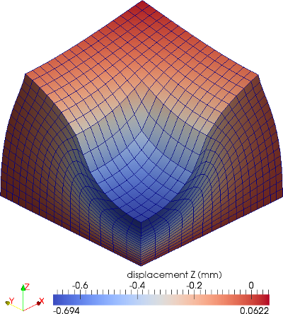
Z-displacement solution for the 3-d problem. | 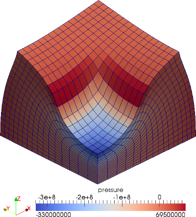
Discontinuous linear pressure field. | 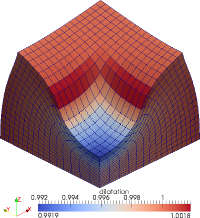
Discontinuous linear dilatation field. |
This brief analysis of the results demonstrates that the three-field formulation is effective in circumventing volumetric locking for highly-incompressible media. The mixed formulation is able to accurately simulate the displacement of a near-incompressible block under compression. The command-line output indicates that the volumetric change under extreme compression resulted in less than 0.01% volume change for a Poisson's ratio of 0.4999.
In terms of run-time, the \(Q_2-DGPM_1-DGPM_1\) formulation tends to be more computationally expensive than the \(Q_1-DGPM_0-DGPM_0\) for a similar number of degrees-of-freedom (produced by adding an extra grid refinement level for the lower-order interpolation). This is shown in the graph below for a batch of tests run consecutively on a single 4-core (8-thread) machine. The increase in computational time for the higher-order method is likely due to the increased band-width required for the higher-order elements. As previously mentioned, the use of a better solver and preconditioner may mitigate the expense of using a higher-order formulation. It was observed that for the given problem using the multithreaded Jacobi preconditioner can reduce the computational runtime by up to 72% (for the worst case being a higher-order formulation with a large number of degrees-of-freedom) in comparison to the single-thread SSOR preconditioner. However, it is the author's experience that the Jacobi method of preconditioning may not be suitable for some finite-strain problems involving alternative constitutive models.
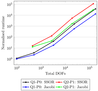
Runtime on a 4-core machine, normalised against the lowest grid resolution \(Q_1-DGPM_0-DGPM_0\) solution that utilised a SSOR preconditioner. |
Lastly, results for the displacement solution for the 2-d problem are showcased below for two different levels of grid refinement. It is clear that due to the extra constraints imposed by simulating in 2-d that the resulting displacement field, although qualitatively similar, is different to that of the 3-d case.
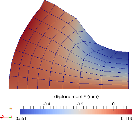
Y-displacement solution in 2-d for 2 global grid refinement levels. | 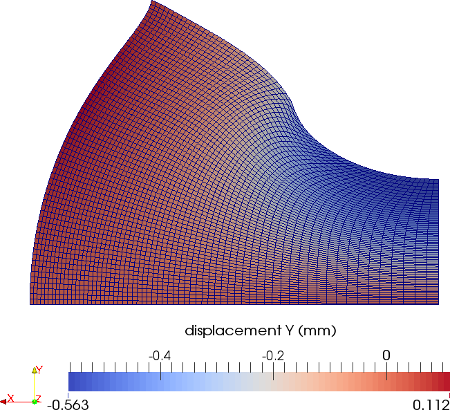
Y-displacement solution in 2-d for 5 global grid refinement levels. |
There are a number of obvious extensions for this work:
PointHistory and linear solver routines. 1.8.14