 |
Reference documentation for deal.II version 9.1.1
|
 |
Reference documentation for deal.II version 9.1.1
|
This tutorial depends on step-13.
| Table of contents | |
|---|---|
The Heidelberg group of Professor Rolf Rannacher, to which the three initial authors of the deal.II library belonged during their PhD time and partly also afterwards, has been involved with adaptivity and error estimation for finite element discretizations since the mid-1990ies. The main achievement is the development of error estimates for arbitrary functionals of the solution, and of optimal mesh refinement for its computation.
We will not discuss the derivation of these concepts in too great detail, but will implement the main ideas in the present example program. For a thorough introduction into the general idea, we refer to the seminal work of Becker and Rannacher [BR95],[BR96r], and the overview article of the same authors in Acta Numerica [BR01]; the first introduces the concept of error estimation and adaptivity for general functional output for the Laplace equation, while the second gives many examples of applications of these concepts to a large number of other, more complicated equations. For applications to individual types of equations, see also the publications by Becker [Bec95], [Bec98], Kanschat [Kan96], [FK97], Suttmeier [Sut96], [RS97], [RS98c], [RS99], Bangerth [BR99b], [Ban00w], [BR01a], [Ban02], and Hartmann [Har02], [HH01], [HH01b]. All of these works, from the original introduction by Becker and Rannacher to individual contributions to particular equations, have later been summarized in a book by Bangerth and Rannacher that covers all of these topics, see [BR03].
The basic idea is the following: in applications, one is not usually interested in the solution per se, but rather in certain aspects of it. For example, in simulations of flow problems, one may want to know the lift or drag of a body immersed in the fluid; it is this quantity that we want to know to best accuracy, and whether the rest of the solution of the describing equations is well resolved is not of primary interest. Likewise, in elasticity one might want to know about values of the stress at certain points to guess whether maximal load values of joints are safe, for example. Or, in radiative transfer problems, mean flux intensities are of interest.
In all the cases just listed, it is the evaluation of a functional J(u) of the solution which we are interested in, rather than the values of u everywhere. Since the exact solution u is not available, but only its numerical approximation u_h, it is sensible to ask whether the computed value J(u_h) is within certain limits of the exact value J(u), i.e. we want to bound the error with respect to this functional, J(u)-J(u_h).
For simplicity of exposition, we henceforth assume that both the quantity of interest J, as well as the equation are linear, and we will in particular show the derivation for the Laplace equation with homogeneous Dirichlet boundary conditions, although the concept is much more general. For this general case, we refer to the references listed above. The goal is to obtain bounds on the error, J(e)=J(u)-J(u_h). For this, let us denote by z the solution of a dual problem, defined as follows:
a(\varphi,z) = J(\varphi) \qquad \forall \varphi,
where a(\cdot,\cdot) is the bilinear form associated with the differential equation, and the test functions are chosen from the corresponding solution space. Then, taking as special test function \varphi=e the error, we have that
J(e) = a(e,z)
and we can, by Galerkin orthogonality, rewrite this as
J(e) = a(e,z-\varphi_h)
where \varphi_h can be chosen from the discrete test space in whatever way we find convenient.
Concretely, for Laplace's equation, the error identity reads
J(e) = (\nabla e, \nabla(z-\varphi_h)).
Because we want to use this formula not only to compute error, but also to refine the mesh, we need to rewrite the expression above as a sum over cells where each cell's contribution can then be used as an error indicator for this cell. Thus, we split the scalar products into terms for each cell, and integrate by parts on each of them:
\begin{eqnarray*} J(e) &=& \sum_K (\nabla (u-u_h), \nabla (z-\varphi_h))_K \\ &=& \sum_K (-\Delta (u-u_h), z-\varphi_h)_K + (\partial_n (u-u_h), z-z_h)_{\partial K}. \end{eqnarray*}
Next we use that -\Delta u=f, and that for solutions of the Laplace equation, the solution is smooth enough that \partial_n u is continuous almost everywhere – so the terms involving \partial_n u on one cell cancels with that on its neighbor, where the normal vector has the opposite sign. (The same is not true for \partial_n u_h, though.) At the boundary of the domain, where there is no neighbor cell with which this term could cancel, the weight z-\varphi_h can be chosen as zero, and the whole term disappears.
Thus, we have
\begin{eqnarray*} J(e) &=& \sum_K (f+\Delta u_h, z-\varphi_h)_K - (\partial_n u_h, z-\varphi_h)_{\partial K\backslash \partial\Omega}. \end{eqnarray*}
In a final step, note that when taking the normal derivative of u_h, we mean the value of this quantity as taken from this side of the cell (for the usual Lagrange elements, derivatives are not continuous across edges). We then rewrite the above formula by exchanging half of the edge integral of cell K with the neighbor cell K', to obtain
\begin{eqnarray*} J(e) &=& \sum_K (f+\Delta u_h, z-\varphi_h)_K - \frac 12 (\partial_n u_h|_K + \partial_{n'} u_h|_{K'}, z-\varphi_h)_{\partial K\backslash \partial\Omega}. \end{eqnarray*}
Using that for the normal vectors on adjacent cells we have n'=-n, we define the jump of the normal derivative by
[\partial_n u_h] \dealcoloneq \partial_n u_h|_K + \partial_{n'} u_h|_{K'} = \partial_n u_h|_K - \partial_n u_h|_{K'},
and get the final form after setting the discrete function \varphi_h, which is by now still arbitrary, to the point interpolation of the dual solution, \varphi_h=I_h z:
\begin{eqnarray*} J(e) &=& \sum_K (f+\Delta u_h, z-I_h z)_K - \frac 12 ([\partial_n u_h], z-I_h z)_{\partial K\backslash \partial\Omega}. \end{eqnarray*}
With this, we have obtained an exact representation of the error of the finite element discretization with respect to arbitrary (linear) functionals J(\cdot). Its structure is a weighted form of a residual estimator, as both f+\Delta u_h and [\partial_n u_h] are cell and edge residuals that vanish on the exact solution, and z-I_h z are weights indicating how important the residuals on a certain cell is for the evaluation of the given functional. Furthermore, it is a cell-wise quantity, so we can use it as a mesh refinement criterion. The question, is: how to evaluate it? After all, the evaluation requires knowledge of the dual solution z, which carries the information about the quantity we want to know to best accuracy.
In some, very special cases, this dual solution is known. For example, if the functional J(\cdot) is the point evaluation, J(\varphi)=\varphi(x_0), then the dual solution has to satisfy
-\Delta z = \delta(x-x_0),
with the Dirac delta function on the right hand side, and the dual solution is the Green's function with respect to the point x_0. For simple geometries, this function is analytically known, and we could insert it into the error representation formula.
However, we do not want to restrict ourselves to such special cases. Rather, we will compute the dual solution numerically, and approximate z by some numerically obtained \tilde z. We note that it is not sufficient to compute this approximation \tilde z using the same method as used for the primal solution u_h, since then \tilde z-I_h \tilde z=0, and the overall error estimate would be zero. Rather, the approximation \tilde z has to be from a larger space than the primal finite element space. There are various ways to obtain such an approximation (see the cited literature), and we will choose to compute it with a higher order finite element space. While this is certainly not the most efficient way, it is simple since we already have all we need to do that in place, and it also allows for simple experimenting. For more efficient methods, again refer to the given literature, in particular [BR95], [BR03].
With this, we end the discussion of the mathematical side of this program and turn to the actual implementation.
The step-14 example program builds heavily on the techniques already used in the step-13 program. Its implementation of the dual weighted residual error estimator explained above is done by deriving a second class, properly called DualSolver, from the Solver base class, and having a class (WeightedResidual) that joins the two again and controls the solution of the primal and dual problem, and then uses both to compute the error indicator for mesh refinement.
The program continues the modular concept of the previous example, by implementing the dual functional, describing quantity of interest, by an abstract base class, and providing two different functionals which implement this interface. Adding a different quantity of interest is thus simple.
One of the more fundamental differences is the handling of data. A common case is that you develop a program that solves a certain equation, and test it with different right hand sides, different domains, different coefficients and boundary values, etc. Usually, these have to match, so that exact solutions are known, or that their combination makes sense at all.
We demonstrate a way how this can be achieved in a simple, yet very flexible way. We will put everything that belongs to a certain setup into one class, and provide a little C++ mortar around it, so that entire setups (domains, coefficients, right hand sides, etc.) can be exchanged by only changing something in one place.
Going this way a little further, we have also centralized all the other parameters that describe how the program is to work in one place, such as the order of the finite element, the maximal number of degrees of freedom, the evaluation objects that shall be executed on the computed solutions, and so on. This allows for simpler configuration of the program, and we will show in a later program how to use a library class that can handle setting these parameters by reading an input file. The general aim is to reduce the places within a program where one may have to look when wanting to change some parameter, as it has turned out in practice that one forgets where they are as programs grow. Furthermore, putting all options describing what the program does in a certain run into a file (that can be stored with the results) helps repeatability of results more than if the various flags were set somewhere in the program, where their exact values are forgotten after the next change to this place.
Unfortunately, the program has become rather long. While this admittedly reduces its usefulness as an example program, we think that it is a very good starting point for development of a program for other kinds of problems, involving different equations than the Laplace equation treated here. Furthermore, it shows everything that we can show you about our way of a posteriori error estimation, and its structure should make it simple for you to adjust this method to other problems, other functionals, other geometries, coefficients, etc.
The author believes that the present program is his masterpiece among the example programs, regarding the mathematical complexity, as well as the simplicity to add extensions. If you use this program as a basis for your own programs, we would kindly like to ask you to state this fact and the name of the author of the example program, Wolfgang Bangerth, in publications that arise from that, of your program consists in a considerable part of the example program.
Wolfgang Bangerth.
Mesh adaptivity and error control for a finite element approximation of the elastic wave equation.
In Alfredo Bermudez, Dolores Gomez, Christophe Hazard, Patrick Joly, and Jean E. Roberts, editors, Proceedings of the Fifth International Conference on Mathematical and Numerical Aspects of Wave Propagation (Waves2000), Santiago de Compostela, Spain, 2000, pages 725–729. SIAM, 2000.
Wolfgang Bangerth.
Adaptive Finite Element Methods for the Identification of Distributed Coefficient in Partial Differential Equations.
PhD thesis, University of Heidelberg, 2002.
Wolfgang Bangerth and Rolf Rannacher.
Finite element approximation of the acoustic wave equation: Error control and mesh adaptation.
East–West J. Numer. Math., 7(4):263–282, 1999.
Wolfgang Bangerth and Rolf Rannacher.
Adaptive Finite Element Methods for Differential Equations.
Birkhäuser Verlag, Basel, 2003.
Wolfgang Bangerth and Rolf Rannacher.
Adaptive finite element techniques for the acoustic wave equation.
J. Comput. Acoustics, 9(2):575–591, 2001.
Roland Becker and Rolf Rannacher.
An optimal control approach to error estimation and mesh adaptation in finite element methods.
Acta Numerica, 10:1–102, 2001.
Roland Becker.
An Adaptive Finite Element Method for the Incompressible Navier-Stokes Equations on Time-dependent Domains.
Dissertation, Universität Heidelberg, 1995.
Roland Becker.
Weighted error estimators for finite element approximations of the incompressible Navier-Stokes equations.
Preprint 98-20, SFB 359, Universität Heidelberg, 1998.
Roland Becker and Rolf Rannacher.
A feed-back approach to error control in finite element methods: Basic analysis and examples.
East–West J. Numer. Math., 4:237–264, 1996.
Roland Becker and Rolf Rannacher.
Weighted a posteriori error control in FE methods.
In H. G. Bock et al., ed.s, ENUMATH 95, pages 621–637, Paris, September 1998. World Scientific Publ., Singapore.
in [enumath97].
Hans Georg Bock, Franco Brezzi, Roland Glowinsky, Guido Kanschat, Yuri A. Kuznetsov, Jacques Periaux, and Rolf Rannacher, editors.
ENUMATH 97, Proceedings of the 2nd European Conference on Numerical Mathematics and Advanced Applications, Singapore, 1998. World Scientific.
Christian Führer and Guido Kanschat.
A posteriori error control in radiative transfer.
Computing, 58(4):317–334, 1997.
Ralf Hartmann.
Adaptive Finite Element Methods for the Compressible Euler Equations.
PhD thesis, University of Heidelberg, 2002.
Ralf Hartmann and Paul Houston.
Adaptive discontinuous Galerkin finite element methods for nonlinear hyperbolic conservation laws.
SIAM J. Sci. Comput., 24 (2002), pp. 979-1004.
Ralf Hartmann and Paul Houston.
Adaptive discontinuous Galerkin finite element methods for the compressible Euler equations.
J. Comput. Phys. 183 (2002), pp. 508-532.
Guido Kanschat.
Parallel and Adaptive Galerkin Methods for Radiative Transfer Problems.
Dissertation, Universität Heidelberg, 1996.
Rolf Rannacher and Franz-Theo Suttmeier.
A feed-back approach to error control in finite element methods: Application to linear elasticity.
Comp. Mech., 19(5):434–446, 1997.
Rolf Rannacher and Franz-Theo Suttmeier.
A posteriori error control in finite element methods via duality techniques: Application to perfect plasticity.
Comp. Mech., 21(2):123–133, 1998.
Rolf Rannacher and Franz-Theo Suttmeier.
A posteriori error control and mesh adaptation for finite element models in elasticity and elasto-plasticity.
Comput. Methods Appl. Mech. Engrg., pages 333–361, 1999.
Franz-Theo Suttmeier.
Adaptive Finite Element Approximation of Problems in Elasto-Plasticity Theory.
Dissertation, Universität Heidelberg, 1996.
Start out with well known things...
The last step is as in all previous programs:
As mentioned in the introduction, significant parts of the program have simply been taken over from the step-13 example program. We therefore only comment on those things that are new.
First, the framework for evaluation of solutions is unchanged, i.e. the base class is the same, and the class to evaluate the solution at a grid point is unchanged:
Besides the class implementing the evaluation of the solution at one point, we here provide one which evaluates the gradient at a grid point. Since in general the gradient of a finite element function is not continuous at a vertex, we have to be a little bit more careful here. What we do is to loop over all cells, even if we have found the point already on one cell, and use the mean value of the gradient at the vertex taken from all adjacent cells.
Given the interface of the PointValueEvaluation class, the declaration of this class provides little surprise, and neither does the constructor:
The more interesting things happen inside the function doing the actual evaluation:
This time initialize the return value with something useful, since we will have to add up a number of contributions and take the mean value afterwards...
...then have some objects of which the meaning will become clear below...
...and next loop over all cells and their vertices, and count how often the vertex has been found:
Things are now no more as simple, since we can't get the gradient of the finite element field as before, where we simply had to pick one degree of freedom at a vertex.
Rather, we have to evaluate the finite element field on this cell, and at a certain point. As you know, evaluating finite element fields at certain points is done through the FEValues class, so we use that. The question is: the FEValues object needs to be a given a quadrature formula and can then compute the values of finite element quantities at the quadrature points. Here, we don't want to do quadrature, we simply want to specify some points!
Nevertheless, the same way is chosen: use a special quadrature rule with points at the vertices, since these are what we are interested in. The appropriate rule is the trapezoidal rule, so that is the reason why we used that one above.
Thus: initialize the FEValues object on this cell,
and extract the gradients of the solution vector at the vertices:
Now we have the gradients at all vertices, so pick out that one which belongs to the evaluation point (note that the order of vertices is not necessarily the same as that of the quadrature points):
Check that the evaluation point was indeed found,
and if so take the x-derivative of the gradient there as the value which we are interested in, and increase the counter indicating how often we have added to that variable:
Finally break out of the innermost loop iterating over the vertices of the present cell, since if we have found the evaluation point at one vertex it cannot be at a following vertex as well:
Now we have looped over all cells and vertices, so check whether the point was found:
We have simply summed up the contributions of all adjacent cells, so we still have to compute the mean value. Once this is done, report the status:
Since this program has a more difficult structure (it computed a dual solution in addition to a primal one), writing out the solution is no more done by an evaluation object since we want to write both solutions at once into one file, and that requires some more information than available to the evaluation classes.
However, we also want to look at the grids generated. This again can be done with one such class. Its structure is analog to the SolutionOutput class of the previous example program, so we do not discuss it here in more detail. Furthermore, everything that is used here has already been used in previous example programs.
Next are the actual solver classes. Again, we discuss only the differences to the previous program.
This class is almost unchanged, with the exception that it declares two more functions: output_solution will be used to generate output files from the actual solutions computed by derived classes, and the set_refinement_cycle function by which the testing framework sets the number of the refinement cycle to a local variable in this class; this number is later used to generate filenames for the solution output.
Likewise, the Solver class is entirely unchanged and will thus not be discussed.
The remainder of the class is essentially a copy of step-13 as well, including the data structures and functions necessary to compute the linear system in parallel using the WorkStream framework:
The following few functions and constructors are verbatim copies taken from step-13:
Now for the functions that implement actions in the linear system class. First, the constructor initializes all data elements to their correct sizes, and sets up a number of additional data structures, such as constraints due to hanging nodes. Since setting up the hanging nodes and finding out about the nonzero elements of the matrix is independent, we do that in parallel (if the library was configured to use concurrency, at least; otherwise, the actions are performed sequentially). Note that we start only one thread, and do the second action in the main thread. Since only one thread is generated, we don't use the Threads::ThreadGroup class here, but rather use the one created thread object directly to wait for this particular thread's exit. The approach is generally the same as the one we have used in Solver::assemble_linear_system() above.
Note that taking the address of the DoFTools::make_hanging_node_constraints function is a little tricky, since there are actually three functions of this name, one for each supported space dimension. Taking addresses of overloaded functions is somewhat complicated in C++, since the address-of operator & in that case returns a set of values (the addresses of all functions with that name), and selecting the right one is then the next step. If the context dictates which one to take (for example by assigning to a function pointer of known type), then the compiler can do that by itself, but if this set of pointers shall be given as the argument to a function that takes a template, the compiler could choose all without having a preference for one. We therefore have to make it clear to the compiler which one we would like to have; for this, we could use a cast, but for more clarity, we assign it to a temporary mhnc_p (short for pointer to make_hanging_node_constraints) with the right type, and using this pointer instead.
Start a side task then continue on the main thread
Wait for the side task to be done before going further
The PrimalSolver class is also mostly unchanged except for implementing the output_solution function. We keep the GlobalRefinement and RefinementKelly classes in this program, and they can then rely on the default implementation of this function which simply outputs the primal solution. The class implementing dual weighted error estimators will overload this function itself, to also output the dual solution.
For the following two classes, the same applies as for most of the above: the class is taken from the previous example as-is:
This class is a variant of the previous one, in that it allows to weight the refinement indicators we get from the library's Kelly indicator by some function. We include this class since the goal of this example program is to demonstrate automatic refinement criteria even for complex output quantities such as point values or stresses. If we did not solve a dual problem and compute the weights thereof, we would probably be tempted to give a hand-crafted weighting to the indicators to account for the fact that we are going to evaluate these quantities. This class accepts such a weighting function as argument to its constructor:
Now, here comes the main function, including the weighting:
First compute some residual based error indicators for all cells by a method already implemented in the library. What exactly we compute here is described in more detail in the documentation of that class.
Next weigh each entry in the vector of indicators by the value of the function given to the constructor, evaluated at the cell center. We need to write the result into the vector entry that corresponds to the current cell, which we can obtain by asking the cell what its index among all active cells is using CellAccessor::active_cell_index(). (In reality, this index is zero for the first cell we handle in the loop, one for the second cell, etc., and we could as well just keep track of this index using an integer counter; but using CellAccessor::active_cell_index() makes this more explicit.)
In this example program, we work with the same data sets as in the previous one, but as it may so happen that someone wants to run the program with different boundary values and right hand side functions, or on a different grid, we show a simple technique to do exactly that. For more clarity, we furthermore pack everything that has to do with equation data into a namespace of its own.
The underlying assumption is that this is a research program, and that there we often have a number of test cases that consist of a domain, a right hand side, boundary values, possibly a specified coefficient, and a number of other parameters. They often vary all at the same time when shifting from one example to another. To make handling such sets of problem description parameters simple is the goal of the following.
Basically, the idea is this: let us have a structure for each set of data, in which we pack everything that describes a test case: here, these are two subclasses, one called BoundaryValues for the boundary values of the exact solution, and one called RightHandSide, and then a way to generate the coarse grid. Since the solution of the previous example program looked like curved ridges, we use this name here for the enclosing class. Note that the names of the two inner classes have to be the same for all enclosing test case classes, and also that we have attached the dimension template argument to the enclosing class rather than to the inner ones, to make further processing simpler. (From a language viewpoint, a namespace would be better to encapsulate these inner classes, rather than a structure. However, namespaces cannot be given as template arguments, so we use a structure to allow a second object to select from within its given argument. The enclosing structure, of course, has no member variables apart from the classes it declares, and a static function to generate the coarse mesh; it will in general never be instantiated.)
The idea is then the following (this is the right time to also take a brief look at the code below): we can generate objects for boundary values and right hand side by simply giving the name of the outer class as a template argument to a class which we call here Data::SetUp, and it then creates objects for the inner classes. In this case, to get all that characterizes the curved ridge solution, we would simply generate an instance of Data::SetUp<Data::CurvedRidge>, and everything we need to know about the solution would be static member variables and functions of that object.
This approach might seem like overkill in this case, but will become very handy once a certain set up is not only characterized by Dirichlet boundary values and a right hand side function, but in addition by material properties, Neumann values, different boundary descriptors, etc. In that case, the SetUp class might consist of a dozen or more objects, and each descriptor class (like the CurvedRidges class below) would have to provide them. Then, you will be happy to be able to change from one set of data to another by only changing the template argument to the SetUp class at one place, rather than at many.
With this framework for different test cases, we are almost finished, but one thing remains: by now we can select statically, by changing one template argument, which data set to choose. In order to be able to do that dynamically, i.e. at run time, we need a base class. This we provide in the obvious way, see below, with virtual abstract functions. It forces us to introduce a second template parameter dim which we need for the base class (which could be avoided using some template magic, but we omit that), but that's all.
Adding new testcases is now simple, you don't have to touch the framework classes, only a structure like the CurvedRidges one is needed.
Based on the above description, the SetUpBase class then looks as follows. To allow using the SmartPointer class with this class, we derived from the Subscriptor class.
And now for the derived class that takes the template argument as explained above.
Here we pack the data elements into private variables, and allow access to them through the methods of the base class.
We have to provide definitions for the static member variables of the above class:
And definitions of the member functions:
The class that is used to describe the boundary values and right hand side of the curved ridge problem already used in the step-13 example program is then like so:
This example program was written while giving practical courses for a lecture on adaptive finite element methods and duality based error estimates. For these courses, we had one exercise, which required to solve the Laplace equation with constant right hand side on a square domain with a square hole in the center, and zero boundary values. Since the implementation of the properties of this problem is so particularly simple here, lets do it. As the number of the exercise was 2.3, we take the liberty to retain this name for the class as well.
We need a class to denote the boundary values of the problem. In this case, this is simple: it's the zero function, so don't even declare a class, just an alias:
Second, a class that denotes the right hand side. Since they are constant, just subclass the corresponding class of the library and be done:
Finally a function to generate the coarse grid. This is somewhat more complicated here, see immediately below.
As stated above, the grid for this example is the square [-1,1]^2 with the square [-1/2,1/2]^2 as hole in it. We create the coarse grid as 4 times 4 cells with the middle four ones missing. To understand how exactly the mesh is going to look, it may be simplest to just look at the "Results" section of this tutorial program first. In general, if you'd like to understand more about creating meshes either from scratch by hand, as we do here, or using other techniques, you should take a look at step-49.
Of course, the example has an extension to 3d, but since this function cannot be written in a dimension independent way we choose not to implement this here, but rather only specialize the template for dim=2. If you compile the program for 3d, you'll get a message from the linker that this function is not implemented for 3d, and needs to be provided.
For the creation of this geometry, the library has no predefined method. In this case, the geometry is still simple enough to do the creation by hand, rather than using a mesh generator.
We first define the space dimension, to allow those parts of the function that are actually dimension independent to use this variable. That makes it simpler if you later take this as a starting point to implement a 3d version of this mesh. The next step is then to have a list of vertices. Here, they are 24 (5 times 5, with the middle one omitted). It is probably best to draw a sketch here.
Next, we have to define the cells and the vertices they contain.
Again, we generate a C++ vector type from this, but this time by looping over the cells (yes, this is boring). Additionally, we set the material indicator to zero for all the cells:
Finally pass all this information to the library to generate a triangulation. The last parameter may be used to pass information about non-zero boundary indicators at certain faces of the triangulation to the library, but we don't want that here, so we give an empty object:
And since we want that the evaluation point (3/4,3/4) in this example is a grid point, we refine once globally:
As you have now read through this framework, you may be wondering why we have not chosen to implement the classes implementing a certain setup (like the CurvedRidges class) directly as classes derived from Data::SetUpBase. Indeed, we could have done very well so. The only reason is that then we would have to have member variables for the solution and right hand side classes in the CurvedRidges class, as well as member functions overloading the abstract functions of the base class giving access to these member variables. The SetUp class has the sole reason to relieve us from the need to reiterate these member variables and functions that would be necessary in all such classes. In some way, the template mechanism here only provides a way to have default implementations for a number of functions that depend on external quantities and can thus not be provided using normal virtual functions, at least not without the help of templates.
However, there might be good reasons to actually implement classes derived from Data::SetUpBase, for example if the solution or right hand side classes require constructors that take arguments, which the Data::SetUpBase class cannot provide. In that case, subclassing is a worthwhile strategy. Other possibilities for special cases are to derive from Data::SetUp<SomeSetUp> where SomeSetUp denotes a class, or even to explicitly specialize Data::SetUp<SomeSetUp>. The latter allows to transparently use the way the SetUp class is used for other set-ups, but with special actions taken for special arguments.
A final observation favoring the approach taken here is the following: we have found numerous times that when starting a project, the number of parameters (usually boundary values, right hand side, coarse grid, just as here) was small, and the number of test cases was small as well. One then starts out by handcoding them into a number of switch statements. Over time, projects grow, and so does the number of test cases. The number of switch statements grows with that, and their length as well, and one starts to find ways to consider impossible examples where domains, boundary values, and right hand sides do not fit together any more, and starts losing the overview over the whole structure. Encapsulating everything belonging to a certain test case into a structure of its own has proven worthwhile for this, as it keeps everything that belongs to one test case in one place. Furthermore, it allows to put these things all in one or more files that are only devoted to test cases and their data, without having to bring their actual implementation into contact with the rest of the program.
As with the other components of the program, we put everything we need to describe dual functionals into a namespace of its own, and define an abstract base class that provides the interface the class solving the dual problem needs for its work.
We will then implement two such classes, for the evaluation of a point value and of the derivative of the solution at that point. For these functionals we already have the corresponding evaluation objects, so they are complementary.
First start with the base class for dual functionals. Since for linear problems the characteristics of the dual problem play a role only in the right hand side, we only need to provide for a function that assembles the right hand side for a given discretization:
As a first application, we consider the functional corresponding to the evaluation of the solution's value at a given point which again we assume to be a vertex. Apart from the constructor that takes and stores the evaluation point, this class consists only of the function that implements assembling the right hand side.
As for doing the main purpose of the class, assembling the right hand side, let us first consider what is necessary: The right hand side of the dual problem is a vector of values J(phi_i), where J is the error functional, and phi_i is the i-th shape function. Here, J is the evaluation at the point x0, i.e. J(phi_i)=phi_i(x0).
Now, we have assumed that the evaluation point is a vertex. Thus, for the usual finite elements we might be using in this program, we can take for granted that at such a point exactly one shape function is nonzero, and in particular has the value one. Thus, we set the right hand side vector to all-zeros, then seek for the shape function associated with that point and set the corresponding value of the right hand side vector to one:
So, first set everything to zeros...
...then loop over cells and find the evaluation point among the vertices (or very close to a vertex, which may happen due to floating point round-off):
Ok, found, so set corresponding entry, and leave function since we are finished:
Finally, a sanity check: if we somehow got here, then we must have missed the evaluation point, so raise an exception unconditionally:
As second application, we again consider the evaluation of the x-derivative of the solution at one point. Again, the declaration of the class, and the implementation of its constructor is not too interesting:
What is interesting is the implementation of this functional: here, J(phi_i)=d/dx phi_i(x0).
We could, as in the implementation of the respective evaluation object take the average of the gradients of each shape function phi_i at this evaluation point. However, we take a slightly different approach: we simply take the average over all cells that surround this point. The question which cells surrounds the evaluation point is made dependent on the mesh width by including those cells for which the distance of the cell's midpoint to the evaluation point is less than the cell's diameter.
Taking the average of the gradient over the area/volume of these cells leads to a dual solution which is very close to the one which would result from the point evaluation of the gradient. It is simple to justify theoretically that this does not change the method significantly.
Again, first set all entries to zero:
Initialize a FEValues object with a quadrature formula, have abbreviations for the number of quadrature points and shape functions...
...and have two objects that are used to store the global indices of the degrees of freedom on a cell, and the values of the gradients of the shape functions at the quadrature points:
Finally have a variable in which we will sum up the area/volume of the cells over which we integrate, by integrating the unit functions on these cells:
Then start the loop over all cells, and select those cells which are close enough to the evaluation point:
If we have found such a cell, then initialize the FEValues object and integrate the x-component of the gradient of each shape function, as well as the unit function for the total area/volume.
If we have the local contributions, distribute them to the global vector:
After we have looped over all cells, check whether we have found any at all, by making sure that their volume is non-zero. If not, then the results will be botched, as the right hand side should then still be zero, so throw an exception:
Finally, we have by now only integrated the gradients of the shape functions, not taking their mean value. We fix this by dividing by the measure of the volume over which we have integrated:
In the same way as the PrimalSolver class above, we now implement a DualSolver. It has all the same features, the only difference is that it does not take a function object denoting a right hand side object, but now takes a DualFunctionalBase object that will assemble the right hand side vector of the dual problem. The rest of the class is rather trivial.
Since both primal and dual solver will use the same triangulation, but different discretizations, it now becomes clear why we have made the Base class a virtual one: since the final class will be derived from both PrimalSolver as well as DualSolver, it would have two Base instances, would we not have marked the inheritance as virtual. Since in many applications the base class would store much more information than just the triangulation which needs to be shared between primal and dual solvers, we do not usually want to use two such base classes.
Here finally comes the main class of this program, the one that implements the dual weighted residual error estimator. It joins the primal and dual solver classes to use them for the computation of primal and dual solutions, and implements the error representation formula for use as error estimate and mesh refinement.
The first few of the functions of this class are mostly overriders of the respective functions of the base class:
In the private section, we have two functions that are used to call the solve_problem functions of the primal and dual base classes. These two functions will be called in parallel by the solve_problem function of this class.
Then declare abbreviations for active cell iterators, to avoid that we have to write this lengthy name over and over again:
Next, declare a data type that we will us to store the contribution of faces to the error estimator. The idea is that we can compute the face terms from each of the two cells to this face, as they are the same when viewed from both sides. What we will do is to compute them only once, based on some rules explained below which of the two adjacent cells will be in charge to do so. We then store the contribution of each face in a map mapping faces to their values, and only collect the contributions for each cell by looping over the cells a second time and grabbing the values from the map.
The data type of this map is declared here:
In the computation of the error estimates on cells and faces, we need a number of helper objects, such as FEValues and FEFaceValues functions, but also temporary objects storing the values and gradients of primal and dual solutions, for example. These fields are needed in the three functions that do the integration on cells, and regular and irregular faces, respectively.
There are three reasonable ways to provide these fields: first, as local variables in the function that needs them; second, as member variables of this class; third, as arguments passed to that function.
These three alternatives all have drawbacks: the third that their number is not negligible and would make calling these functions a lengthy enterprise. The second has the drawback that it disallows parallelization, since the threads that will compute the error estimate have to have their own copies of these variables each, so member variables of the enclosing class will not work. The first approach, although straightforward, has a subtle but important drawback: we will call these functions over and over again, many thousands of times maybe; it now turns out that allocating vectors and other objects that need memory from the heap is an expensive business in terms of run-time, since memory allocation is expensive when several threads are involved. It is thus significantly better to allocate the memory only once, and recycle the objects as often as possible.
What to do? Our answer is to use a variant of the third strategy. In fact, this is exactly what the WorkStream concept is supposed to do (we have already introduced it above, but see also Parallel computing with multiple processors accessing shared memory). To avoid that we have to give these functions a dozen or so arguments, we pack all these variables into two structures, one which is used for the computations on cells, the other doing them on the faces. Both are then joined into the WeightedResidualScratchData class that will serve as the "scratch data" class of the WorkStream concept:
WorkStream::run generally wants both a scratch object and a copy object. Here, for reasons similar to what we had in step-9 when discussing the computation of an approximation of the gradient, we don't actually need a "copy data" structure. Since WorkStream insists on having one of these, we just declare an empty structure that does nothing other than being there.
Regarding the evaluation of the error estimator, we have one driver function that uses WorkStream::run() to call the second function on every cell:
Then we have functions that do the actual integration of the error representation formula. They will treat the terms on the cell interiors, on those faces that have no hanging nodes, and on those faces with hanging nodes, respectively:
In the implementation of this class, we first have the constructors of the CellData and FaceData member classes, and the WeightedResidual constructor. They only initialize fields to their correct lengths, so we do not have to discuss them in too much detail:
The next five functions are boring, as they simply relay their work to the base classes. The first calls the primal and dual solvers in parallel, while postprocessing the solution and retrieving the number of degrees of freedom is done by the primal class.
Now, it is becoming more interesting: the refine_grid() function asks the error estimator to compute the cell-wise error indicators, then uses their absolute values for mesh refinement.
First call the function that computes the cell-wise and global error:
Then note that marking cells for refinement or coarsening only works if all indicators are positive, to allow their comparison. Thus, drop the signs on all these indicators:
Finally, we can select between different strategies for refinement. The default here is to refine those cells with the largest error indicators that make up for a total of 80 per cent of the error, while we coarsen those with the smallest indicators that make up for the bottom 2 per cent of the error.
Since we want to output both the primal and the dual solution, we overload the output_solution function. The only interesting feature of this function is that the primal and dual solutions are defined on different finite element spaces, which is not the format the DataOut class expects. Thus, we have to transfer them to a common finite element space. Since we want the solutions only to see them qualitatively, we contend ourselves with interpolating the dual solution to the (smaller) primal space. For the interpolation, there is a library function, that takes a AffineConstraints object including the hanging node constraints. The rest is standard.
Add the data vectors for which we want output. Add them both, the DataOut functions can handle as many data vectors as you wish to write to output:
As for the actual computation of error estimates, let's start with the function that drives all this, i.e. calls those functions that actually do the work, and finally collects the results.
The first task in computing the error is to set up vectors that denote the primal solution, and the weights (z-z_h)=(z-I_hz), both in the finite element space for which we have computed the dual solution. For this, we have to interpolate the primal solution to the dual finite element space, and to subtract the interpolation of the computed dual solution to the primal finite element space. Fortunately, the library provides functions for the interpolation into larger or smaller finite element spaces, so this is mostly obvious.
First, let's do that for the primal solution: it is cell-wise interpolated into the finite element space in which we have solved the dual problem: But, again as in the WeightedResidual::output_solution function we first need to create an AffineConstraints object including the hanging node constraints, but this time of the dual finite element space.
Then for computing the interpolation of the numerically approximated dual solution z into the finite element space of the primal solution and subtracting it from z: use the interpolate_difference function, that gives (z-I_hz) in the element space of the dual solution.
Note that this could probably have been more efficient since those constraints have been used previously when assembling matrix and right hand side for the primal problem and writing out the dual solution. We leave the optimization of the program in this respect as an exercise.
Having computed the dual weights we now proceed with computing the cell and face residuals of the primal solution. First we set up a map between face iterators and their jump term contributions of faces to the error estimator. The reason is that we compute the jump terms only once, from one side of the face, and want to collect them only afterwards when looping over all cells a second time.
We initialize this map already with a value of -1e20 for all faces, since this value will stand out in the results if something should go wrong and we fail to compute the value for a face for some reason. Secondly, this initialization already makes the std::map object allocate all objects it may possibly need. This is important since we will write into this structure from parallel threads, and doing so would not be thread-safe if the map needed to allocate memory and thereby reshape its data structures. In other words, the initial initialization relieves us from the necessity to synchronize the threads through a mutex each time they write to (and modify the structure of) this map.
Then hand it all off to WorkStream::run() to compute the estimators for all cells in parallel:
Once the error contributions are computed, sum them up. For this, note that the cell terms are already set, and that only the edge terms need to be collected. Thus, loop over all cells and their faces, make sure that the contributions of each of the faces are there, and add them up. Only take minus one half of the jump term, since the other half will be taken by the neighboring cell.
Next we have the function that is called to estimate the error on a single cell. The function may be called multiple times if the library was configured to use multithreading. Here it goes:
Because of WorkStream, estimate_on_one_cell requires a CopyData object even if it is no used. The next line silences a warning about this unused variable.
First task on each cell is to compute the cell residual contributions of this cell, and put them into the error_indicators variable:
After computing the cell terms, turn to the face terms. For this, loop over all faces of the present cell, and see whether something needs to be computed on it:
First, if this face is part of the boundary, then there is nothing to do. However, to make things easier when summing up the contributions of the faces of cells, we enter this face into the list of faces with a zero contribution to the error.
Next, note that since we want to compute the jump terms on each face only once although we access it twice (if it is not at the boundary), we have to define some rules who is responsible for computing on a face:
First, if the neighboring cell is on the same level as this one, i.e. neither further refined not coarser, then the one with the lower index within this level does the work. In other words: if the other one has a lower index, then skip work on this face:
Likewise, we always work from the coarser cell if this and its neighbor differ in refinement. Thus, if the neighboring cell is less refined than the present one, then do nothing since we integrate over the subfaces when we visit the coarse cell.
Now we know that we are in charge here, so actually compute the face jump terms. If the face is a regular one, i.e. the other side's cell is neither coarser not finer than this cell, then call one function, and if the cell on the other side is further refined, then use another function. Note that the case that the cell on the other side is coarser cannot happen since we have decided above that we handle this case when we pass over that other cell.
As for the actual computation of the error contributions, first turn to the cell terms:
The tasks to be done are what appears natural from looking at the error estimation formula: first get the right hand side and Laplacian of the numerical solution at the quadrature points for the cell residual,
...then get the dual weights...
...and finally build the sum over all quadrature points and store it with the present cell:
On the other hand, computation of the edge terms for the error estimate is not so simple. First, we have to distinguish between faces with and without hanging nodes. Because it is the simple case, we first consider the case without hanging nodes on a face (let's call this the ‘regular’ case):
The first step is to get the values of the gradients at the quadrature points of the finite element field on the present cell. For this, initialize the FEFaceValues object corresponding to this side of the face, and extract the gradients using that object.
The second step is then to extract the gradients of the finite element solution at the quadrature points on the other side of the face, i.e. from the neighboring cell.
For this, do a sanity check before: make sure that the neighbor actually exists (yes, we should not have come here if the neighbor did not exist, but in complicated software there are bugs, so better check this), and if this is not the case throw an error.
If we have that, then we need to find out with which face of the neighboring cell we have to work, i.e. the how-many'th the neighbor the present cell is of the cell behind the present face. For this, there is a function, and we put the result into a variable with the name neighbor_neighbor:
Then define an abbreviation for the neighbor cell, initialize the FEFaceValues object on that cell, and extract the gradients on that cell:
Now that we have the gradients on this and the neighboring cell, compute the jump residual by multiplying the jump in the gradient with the normal vector:
Next get the dual weights for this face:
Finally, we have to compute the sum over jump residuals, dual weights, and quadrature weights, to get the result for this face:
Double check that the element already exists and that it was not already written to...
...then store computed value at assigned location. Note that the stored value does not contain the factor 1/2 that appears in the error representation. The reason is that the term actually does not have this factor if we loop over all faces in the triangulation, but only appears if we write it as a sum over all cells and all faces of each cell; we thus visit the same face twice. We take account of this by using this factor -1/2 later, when we sum up the contributions for each cell individually.
We are still missing the case of faces with hanging nodes. This is what is covered in this function:
First again two abbreviations, and some consistency checks whether the function is called only on faces for which it is supposed to be called:
Then find out which neighbor the present cell is of the adjacent cell. Note that we will operate on the children of this adjacent cell, but that their orientation is the same as that of their mother, i.e. the neighbor direction is the same.
Then simply do everything we did in the previous function for one face for all the sub-faces now:
Start with some checks again: get an iterator pointing to the cell behind the present subface and check whether its face is a subface of the one we are considering. If that were not the case, then there would be either a bug in the neighbor_neighbor function called above, or – worse – some function in the library did not keep to some underlying assumptions about cells, their children, and their faces. In any case, even though this assertion should not be triggered, it does not harm to be cautious, and in optimized mode computations the assertion will be removed anyway.
Now start the work by again getting the gradient of the solution first at this side of the interface,
then at the other side,
and finally building the jump residuals. Since we take the normal vector from the other cell this time, revert the sign of the first term compared to the other function:
Then get dual weights:
At last, sum up the contribution of this sub-face, and set it in the global map:
Once the contributions of all sub-faces are computed, loop over all sub-faces to collect and store them with the mother face for simple use when later collecting the error terms of cells. Again make safety checks that the entries for the sub-faces have been computed and do not carry an invalid value.
Finally store the value with the parent face.
In the previous example program, we have had two functions that were used to drive the process of solving on subsequently finer grids. We extend this here to allow for a number of parameters to be passed to these functions, and put all of that into framework class.
You will have noted that this program is built up of a number of small parts (evaluation functions, solver classes implementing various refinement methods, different dual functionals, different problem and data descriptions), which makes the program relatively simple to extend, but also allows to solve a large number of different problems by replacing one part by another. We reflect this flexibility by declaring a structure in the following framework class that holds a number of parameters that may be set to test various combinations of the parts of this program, and which can be used to test it at various problems and discretizations in a simple way.
First, we declare two abbreviations for simple use of the respective data types:
Then we have the structure which declares all the parameters that may be set. In the default constructor of the structure, these values are all set to default values, for simple use.
First allow for the degrees of the piecewise polynomials by which the primal and dual problems will be discretized. They default to (bi-, tri-)linear ansatz functions for the primal, and (bi-, tri-)quadratic ones for the dual problem. If a refinement criterion is chosen that does not need the solution of a dual problem, the value of the dual finite element degree is of course ignored.
Then have an object that describes the problem type, i.e. right hand side, domain, boundary values, etc. The pointer needed here defaults to the Null pointer, i.e. you will have to set it in actual instances of this object to make it useful.
Since we allow to use different refinement criteria (global refinement, refinement by the Kelly error indicator, possibly with a weight, and using the dual estimator), define a number of enumeration values, and subsequently a variable of that type. It will default to dual_weighted_error_estimator.
Next, an object that describes the dual functional. It is only needed if the dual weighted residual refinement is chosen, and also defaults to a Null pointer.
Then a list of evaluation objects. Its default value is empty, i.e. no evaluation objects.
Next to last, a function that is used as a weight to the RefinementWeightedKelly class. The default value of this pointer is zero, but you have to set it to some other value if you want to use the weighted_kelly_indicator refinement criterion.
Finally, we have a variable that denotes the maximum number of degrees of freedom we allow for the (primal) discretization. If it is exceeded, we stop the process of solving and intermittent mesh refinement. Its default value is 20,000.
Finally the default constructor of this class:
The driver framework class only has one method which calls solver and mesh refinement intermittently, and does some other small tasks in between. Since it does not need data besides the parameters given to it, we make it static:
As for the implementation, first the constructor of the parameter object, setting all values to their defaults:
Then the function which drives the whole process:
First create a triangulation from the given data object,
then a set of finite elements and appropriate quadrature formula:
Next, select one of the classes implementing different refinement criteria.
Now that all objects are in place, run the main loop. The stopping criterion is implemented at the bottom of the loop.
In the loop, first set the new cycle number, then solve the problem, output its solution(s), apply the evaluation objects to it, then decide whether we want to refine the mesh further and solve again on this mesh, or jump out of the loop.
Clean up the screen after the loop has run:
Here finally comes the main function. It drives the whole process by specifying a set of parameters to be used for the simulation (polynomial degrees, evaluation and dual functionals, etc), and passes them packed into a structure to the frame work class above.
Describe the problem we want to solve here by passing a descriptor object to the function doing the rest of the work:
First set the refinement criterion we wish to use:
Here, we could as well have used global_refinement or weighted_kelly_indicator. Note that the information given about dual finite elements, dual functional, etc is only important for the given choice of refinement criterion, and is ignored otherwise.
Then set the polynomial degrees of primal and dual problem. We choose here bi-linear and bi-quadratic ones:
Then set the description of the test case, i.e. domain, boundary values, and right hand side. These are prepackaged in classes. We take here the description of Exercise_2_3, but you can also use CurvedRidges<dim>:
Next set first a dual functional, then a list of evaluation objects. We choose as default the evaluation of the value at an evaluation point, represented by the classes PointValueEvaluation in the namespaces of evaluation and dual functional classes. You can also set the PointXDerivativeEvaluation classes for the x-derivative instead of the value at the evaluation point.
Note that dual functional and evaluation objects should match. However, you can give as many evaluation functionals as you want, so you can have both point value and derivative evaluated after each step. One such additional evaluation is to output the grid in each step.
Set the maximal number of degrees of freedom after which we want the program to stop refining the mesh further:
Finally pass the descriptor object to a function that runs the entire solution with it:
Catch exceptions to give information about things that failed:
This program offers a lot of possibilities to play around. We can thus only show a small part of all possible results that can be obtained with the help of this program. However, you are encouraged to just try it out, by changing the settings in the main program. Here, we start by simply letting it run, unmodified:
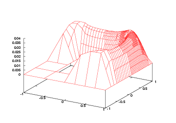
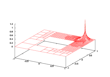
First let's look what the program actually computed. On the fifth grid, primal and dual numerical solutions look like this:
| 
|
Obviously, the region at the bottom left is so unimportant for the point value evaluation at the top right that the grid is left entirely unrefined there, even though the solution has singularities there! Due to the symmetry in right hand side and domain, the solution should actually look like at the top right in all four corners, but the mesh refinement criterion involving the dual solution chose to refine them differently.
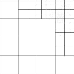
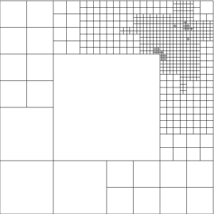
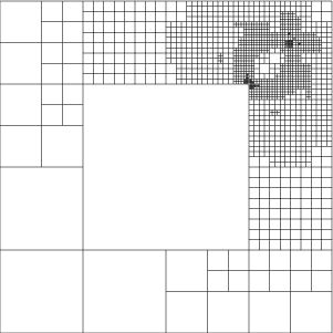
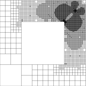
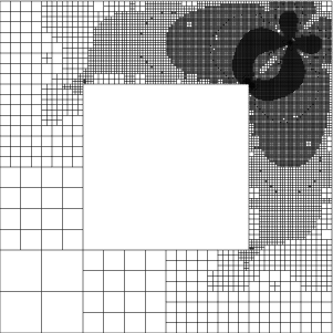
Looking at the grids that are produced in the course of subsequent refinement, here are some of them:

| 
| 
|
| 
| 
|
Note the subtle interplay between resolving the corner singularities, and resolving around the point of evaluation. It will be rather difficult to generate such a mesh by hand, as this would involve to judge quantitatively how much which of the four corner singularities shall be resolved, and to set the weight compared to the vicinity of the evaluation point.
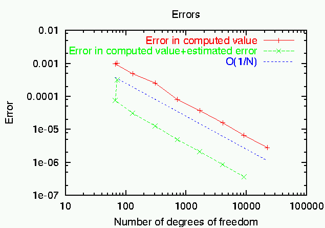
The program prints the point value and the estimated error in this quantity. From extrapolating it, we can guess that the exact value is somewhat like 0.0334473, plus or minus 0.0000001 (note that we get almost 6 valid digits from only 22,000 (primal) degrees of freedom. This number cannot be obtained from the value of the functional alone, but I have used the assumption that the error estimator is mostly exact, and extrapolated the computed value plus the estimated error, to get an approximation of the true value. Computing with more degrees of freedom shows that this assumption is indeed valid.
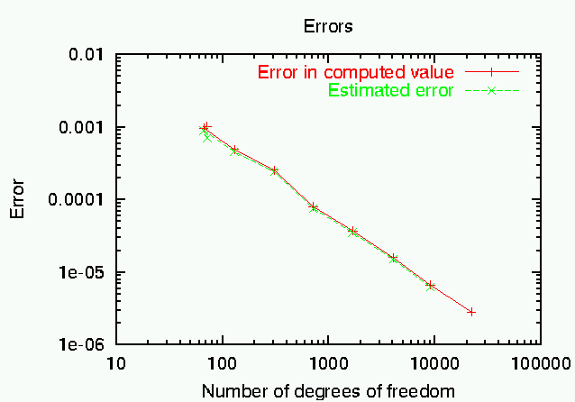
From the computed results, we can generate two graphs: one that shows the convergence of the error J(u)-J(u_h) (taking the extrapolated value as correct) in the point value, and the value that we get by adding up computed value J(u_h) and estimated error eta (if the error estimator eta were exact, then the value J(u_h)+\eta would equal the exact point value, and the error in this quantity would always be zero; however, since the error estimator is only a - good - approximation to the true error, we can by this only reduce the size of the error). In this graph, we also indicate the complexity {\cal O}(1/N) to show that mesh refinement acts optimal in this case. The second chart compares true and estimated error, and shows that the two are actually very close to each other, even for such a complicated quantity as the point value:
| 
|
Since we have accepted quite some effort when using the mesh refinement driven by the dual weighted error estimator (for solving the dual problem, and for evaluating the error representation), it is worth while asking whether that effort was successful. To this end, we first compare the achieved error levels for different mesh refinement criteria. To generate this data, simply change the value of the mesh refinement criterion variable in the main program. The results are thus (for the weight in the Kelly indicator, we have chosen the function 1/(r^2+0.1^2), where r is the distance to the evaluation point; it can be shown that this is the optimal weight if we neglect the effects of boundaries):
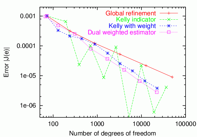
Checking these numbers, we see that for global refinement, the error is proportional to O(1/(sqrt(N) log(N))), and for the dual estimator O(1/N). Generally speaking, we see that the dual weighted error estimator is better than the other refinement indicators, at least when compared with those that have a similarly regular behavior. The Kelly indicator produces smaller errors, but jumps about the picture rather irregularly, with the error also changing signs sometimes. Therefore, its behavior does not allow to extrapolate the results to larger values of N. Furthermore, if we trust the error estimates of the dual weighted error estimator, the results can be improved by adding the estimated error to the computed values. In terms of reliability, the weighted estimator is thus better than the Kelly indicator, although the latter sometimes produces smaller errors.
Besides evaluating the values of the solution at a certain point, the program also offers the possibility to evaluate the x-derivatives at a certain point, and also to tailor mesh refinement for this. To let the program compute these quantities, simply replace the two occurrences of PointValueEvaluation in the main function by PointXDerivativeEvaluation, and let the program run:
The solution looks roughly the same as before (the exact solution of course is the same, only the grid changed a little), but the dual solution is now different. A close-up around the point of evaluation shows this:
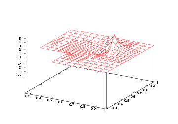
|
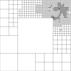
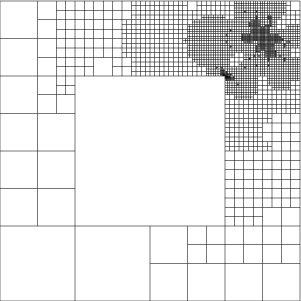
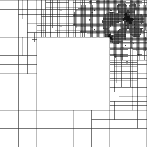
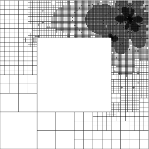
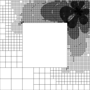
This time, the grids in refinement cycles 0, 5, 6, 7, 8, and 9 look like this:

| 
| 
|
| 
| 
|
Note the asymmetry of the grids compared with those we obtained for the point evaluation, which is due to the directionality of the x-derivative for which we tailored the refinement criterion.
Then, it is interesting to compare actually computed values of the quantity of interest (i.e. the x-derivative of the solution at one point) with a reference value of -0.0528223... plus or minus 0.0000005. We get this reference value by computing on finer grid after some more mesh refinements, with approximately 130,000 cells. Recall that if the error is O(1/N) in the optimal case, then taking a mesh with ten times more cells gives us one additional digit in the result.
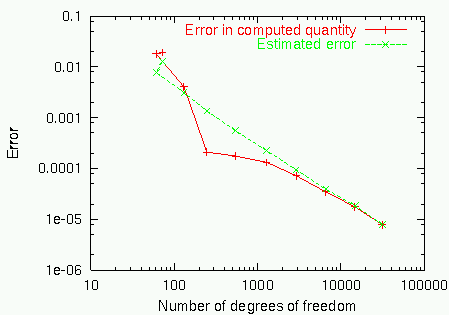
In the left part of the following chart, you again see the convergence of the error towards this extrapolated value, while on the right you see a comparison of true and estimated error:
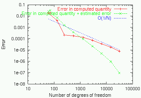
| 
|
After an initial phase where the true error changes its sign, the estimated error matches it quite well, again. Also note the dramatic improvement in the error when using the estimated error to correct the computed value of J(u_h).
If instead of the Exercise_2_3 data set, we choose CurvedRidges in the main function, we can redo the computations of the previous example program, to compare whether the results obtained with the help of the dual weighted error estimator are better than those we had previously.
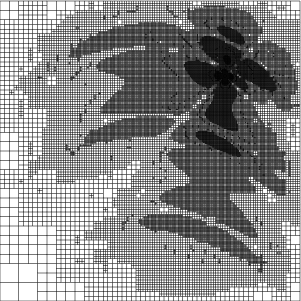
First, the meshes after 9 and 10 adaptive refinement cycles, respectively, look like this:
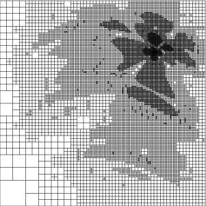
| 
|
The features of the solution can still be seen slightly, but since the solution is smooth, the roughness of the dual solution entirely dominates the mesh refinement criterion, and leads to strongly concentrated meshes. The solution after the seventh refinement step is like so:
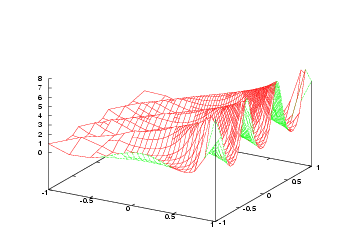
|
Obviously, the solution is worse at some places, but the mesh refinement process should have taken care that these places are not important for computing the point value.
The next point is to compare the new (duality based) mesh refinement criterion with the old ones. These are the results:
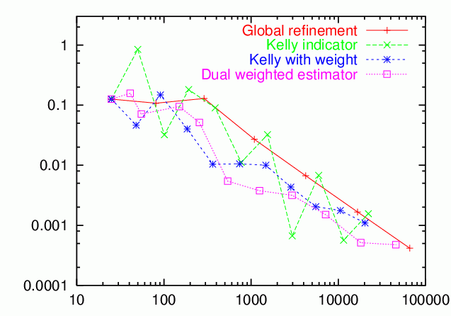
The results are, well, somewhat mixed. First, the Kelly indicator disqualifies itself by its unsteady behavior, changing the sign of the error several times, and with increasing errors under mesh refinement. The dual weighted error estimator has a monotone decrease in the error, and is better than the weighted Kelly and global refinement, but the margin is not as large as expected. This is, here, due to the fact the global refinement can exploit the regular structure of the meshes around the point of evaluation, which leads to a better order of convergence for the point error. However, if we had a mesh that is not locally rectangular, for example because we had to approximate curved boundaries, or if the coefficients were not constant, then this advantage of globally refinement meshes would vanish, while the good performance of the duality based estimator would remain.
The results here are not too clearly indicating the superiority of the dual weighted error estimation approach for mesh refinement over other mesh refinement criteria, such as the Kelly indicator. This is due to the relative simplicity of the shown applications. If you are not convinced yet that this approach is indeed superior, you are invited to browse through the literature indicated in the introduction, where plenty of examples are provided where the dual weighted approach can reduce the necessary numerical work by orders of magnitude, making this the only way to compute certain quantities to reasonable accuracies at all.
Besides the objections you may raise against its use as a mesh refinement criterion, consider that accurate knowledge of the error in the quantity one might want to compute is of great use, since we can stop computations when we are satisfied with the accuracy. Using more traditional approaches, it is very difficult to get accurate estimates for arbitrary quantities, except for, maybe, the error in the energy norm, and we will then have no guarantee that the result we computed satisfies any requirements on its accuracy. Also, as was shown for the evaluation of point values and derivatives, the error estimate can be used to extrapolate the results, yielding much higher accuracy in the quantity we want to know.
Leaving these mathematical considerations, we tried to write the program in a modular way, such that implementing another test case, or another evaluation and dual functional is simple. You are encouraged to take the program as a basis for your own experiments, and to play a little.
 1.8.14