 |
Reference documentation for deal.II version 9.2.0
|
 |
Reference documentation for deal.II version 9.2.0
|
This tutorial depends on step-1.
| Table of contents | |
|---|---|
This tutorial is an extension to step-1 and demonstrates several ways to obtain more involved meshes than the ones shown there.
Generating complex geometries is a challenging task, especially in three space dimensions. We will discuss several ways to do this, but this list is not exhaustive. Additionally, there is not one approach that fits all problems.
This example program shows some of ways to create and modify meshes for computations and outputs them as .vtu files in much the same way as we do in step-1. No other computations or adaptive refinements are done; the idea is that you can use the techniques used here as building blocks in other, more involved simulators. Please note that the example program does not show all the ways to generate meshes that are discussed in this introduction.
When you use adaptive mesh refinement, you definitely want the initial mesh to be as coarse as possible. The reason is that you can make it as fine as you want using adaptive refinement as long as you have memory and CPU time available. However, this requires that you don't waste mesh cells in parts of the domain where they don't pay off. As a consequence, you don't want to start with a mesh that is too fine to start with, because that takes up a good part of your cell budget already, and because you can't coarsen away cells that are in the initial mesh.
That said, your mesh needs to capture the given geometry adequately.
There are several ways to create an initial mesh. Meshes can be modified or combined in many ways as discussed later on.
The easiest way to generate meshes is to use the functions in namespace GridGenerator, as already discussed in step-1. There are many different helper functions available, including GridGenerator::hyper_cube(), GridGenerator::hyper_shell(), GridGenerator::hyper_ball(), and GridGenerator::hyper_cube_with_cylindrical_hole().
If there is no good fit in the GridGenerator namespace for what you want to do, you can always create a Triangulation in your program "by hand". For that, you need a list of vertices with their coordinates and a list of cells referencing those vertices. You can find an example in the function create_coarse_grid() in step-14. All the functions in GridGenerator are implemented in this fashion.
We are happy to accept more functions to be added to GridGenerator. So, if you end up writing a function that might be useful for a larger audience, please contribute it.
The class GridIn can read many different mesh formats from a file from disk. How this is done is explained in step-5 and can be seen in the function grid_1 in this example, see the code below.
Meshes can be generated from different tools like gmsh, lagrit and cubit. See the documentation of GridIn for more information. The problem is that deal.II needs meshes that only consist of quadrilaterals and hexahedra – tetrahedral meshes won't work (this means tools like tetgen can not be used directly).
We will describe a possible workflow using Gmsh. Gmsh is the smallest and most quickly set up open source tool we are aware of. It can generate unstructured 2d quad meshes. In 3d, it can extrude 2d meshes to get hexahedral meshes; 3D meshing of unstructured geometry into hexahedra is possible, though there are some issues with the quality of these meshes that imply that these meshes only sometimes work in deal.II.
In Gmsh, a mesh is fundamentally described in a text-based .geo file whose format can contain computations, loops, variables, etc. This format is quite flexible in allowing the description of complex geometries. The mesh is then generated from a surface representation, which is built from a list of line loops, which is built from a list of lines, which are in turn built from points. The .geo script can be written and edited by hand or it can be generated automatically by creating objects graphically inside Gmsh. In many cases it is best to combine both approaches. The file can be easily reloaded by pressing "reload" under the "Geometry" tab if you want to write it by hand and see the effects in the graphical user interface of gmsh.
This tutorial contains an example .geo file that describes a box with two objects cut out in the interior. This is how example.geo looks like in Gmsh (displaying the boundary indicators as well as the mesh discussed further down below):
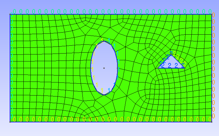
You might want to open the example.geo file in a text editor (it is located in the same directory as the step-49.cc source file) to see how it is structured. You can see how the boundary of the domain is composed of a number of lines and how later on we combine several lines into "physical lines" (or "physical surfaces") that list the logical lines' numbers. "Physical" object are the ones that carry information about the boundary indicator (see this glossary entry).
deal.II's GridIn class can read the .msh format written by Gmsh and that contains a mesh created for the geometry described by the .geo file. You generate the .msh from the .geo by running the commands
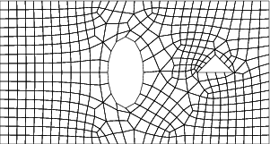
on the command line, or by clicking "Mesh" and then "2D" inside Gmsh after loading the file. Now this is the mesh read from the .msh file and saved again by deal.II as an image (see the grid_1 function of the current program):
.geo file is probably the simplest approach), but instead wants to do parametric studies over the geometry for which it is necessary to generate many meshes for geometries that differ in certain parameters. Another case where this is useful is if there is already a CAD geometry for which one only needs a mesh; indeed, this can be done from within deal.II using the Gmsh::create_triangulation_from_boundary_curve() function.After acquiring one (or several) meshes in the ways described above, there are many ways to manipulate them before using them in a finite element computation.
The GridTools namespace contains a collection of small functions to transform a given mesh in various ways. The usage of the functions GridTools::shift, GridTools::rotate, GridTools::scale is fairly obvious, so we won't discuss those functions here.
The function GridTools::transform allows you to transform the vertices of a given mesh using a smooth function. An example of its use is also given in the results section of step-38 but let us show a simpler example here: In the function grid_5() of the current program, we perturb the y coordinate of a mesh with a sine curve:
 regular input mesh regular input mesh |  output mesh output mesh |
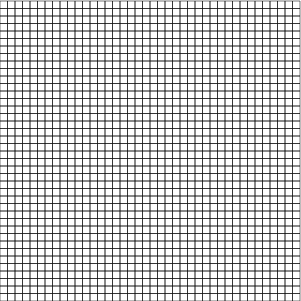
Similarly, we can transform a regularly refined unit square to a wall-adapted mesh in y direction using the formula (x,y) \mapsto (x,\tanh(2 y)/\tanh(2)). This is done in grid_6() of this tutorial:
 regular input mesh regular input mesh | 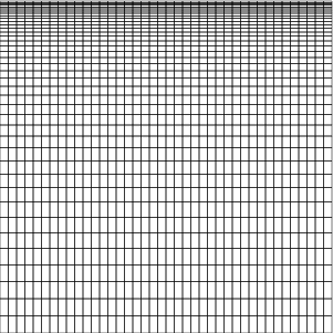 wall-adapted output mesh wall-adapted output mesh |
Finally, the function GridTools::distort_random allows you to move vertices in the mesh (optionally ignoring boundary nodes) by a random amount. This is demonstrated in grid_7() and the result is as follows:
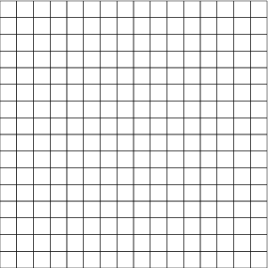 regular input mesh regular input mesh | 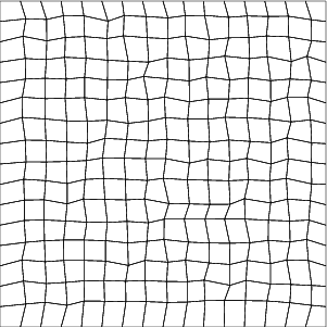 perturbed output mesh perturbed output mesh |
This function is primarily intended to negate some of the superconvergence effects one gets when studying convergence on regular meshes, as well as to suppress some optimizations in deal.II that can exploit the fact that cells are similar in shape. (Superconvergence refers to the fact that if a mesh has certain symmetries – for example, if the edges running into a vertex are symmetric to this vertex, and if this is so for all vertices of a cell – that the solution is then often convergent with a higher order than one would have expected from the usual error analysis. In the end, this is a result of the fact that if one were to make a Taylor expansion of the error, the symmetry leads to the fact that the expected next term of the expansion happens to be zero, and the error order is determined by the second next* term. A distorted mesh does not have these symmetries and consequently the error reflects what one will see when solving the equation on any kind of mesh, rather than showing something that is only reflective of a particular situation.)
The function GridGenerator::merge_triangulations() allows you to merge two given Triangulation objects into a single one. For this to work, the vertices of the shared edge or face have to match exactly. Lining up the two meshes can be achieved using GridTools::shift and GridTools::scale. In the function grid_2() of this tutorial, we merge a square with a round hole (generated with GridGenerator::hyper_cube_with_cylindrical_hole()) and a rectangle (generated with GridGenerator::subdivided_hyper_rectangle()). The function GridGenerator::subdivided_hyper_rectangle() allows you to specify the number of repetitions and the positions of the corners, so there is no need to shift the triangulation manually here. You should inspect the mesh graphically to make sure that cells line up correctly and no unpaired nodes exist in the merged Triangulation.
These are the input meshes and the output mesh:
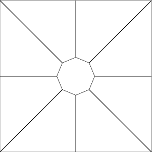 input mesh 1 input mesh 1 | 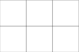 input mesh 2 input mesh 2 | 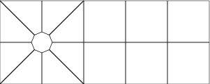 merged mesh merged mesh |
The function grid_3() demonstrates the ability to pick individual vertices and move them around in an existing mesh. Note that this has the potential to produce degenerate or inverted cells and you shouldn't expect anything useful to come of using such meshes. Here, we create a box with a cylindrical hole that is not exactly centered by moving the top vertices upwards:
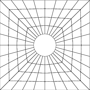 input mesh input mesh | 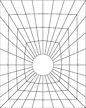 top vertices moved upwards top vertices moved upwards |
For the exact way how this is done, see the code below.
If you need a 3d mesh that can be created by extruding a given 2d mesh (that can be created in any of the ways given above), you can use the function GridGenerator::extrude_triangulation(). See the grid_4() function in this tutorial for an example. Note that for this particular case, the given result could also be achieved using the 3d version of GridGenerator::hyper_cube_with_cylindrical_hole(). The main usage is a 2d mesh, generated for example with Gmsh, that is read in from a .msh file as described above. This is the output from grid_4():
 input mesh input mesh | 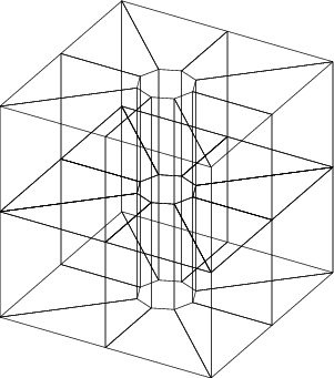 extruded output mesh extruded output mesh |
Creating a coarse mesh using the methods discussed above is only the first step. When you have it, it will typically serve as the basis for further mesh refinement. This is not difficult — in fact, there is nothing else to do — if your geometry consists of only straight faces. However, this is often not the case if you have a more complex geometry and more steps than just creating the mesh are necessary. We will go over some of these steps in the results section below.
This tutorial program is odd in the sense that, unlike for most other steps, the introduction already provides most of the information on how to use the various strategies to generate meshes. Consequently, there is little that remains to be commented on here, and we intersperse the code with relatively little text. In essence, the code here simply provides a reference implementation of what has already been described in the introduction.
The following function generates some output for any of the meshes we will be generating in the remainder of this program. In particular, it generates the following information:
Finally, the function outputs the mesh in VTU format that can easily be visualized in Paraview or VisIt.
Next loop over all faces of all cells and find how often each boundary indicator is used (recall that if you access an element of a std::map object that doesn't exist, it is implicitly created and default initialized – to zero, in the current case – before we then increment it):
Finally, produce a graphical representation of the mesh to an output file :
In this first example, we show how to load the mesh for which we have discussed in the introduction how to generate it. This follows the same pattern as used in step-5 to load a mesh, although there it was written in a different file format (UCD instead of MSH).
Here, we first create two triangulations and then merge them into one. As discussed in the introduction, it is important to ensure that the vertices at the common interface are located at the same coordinates.
In this function, we move vertices of a mesh. This is simpler than one usually expects: if you ask a cell using cell->vertex(i) for the coordinates of its ith vertex, it doesn't just provide the location of this vertex but in fact a reference to the location where these coordinates are stored. We can then modify the value stored there.
So this is what we do in the first part of this function: We create a square of geometry [-1,1]^2 with a circular hole with radius 0.25 located at the origin. We then loop over all cells and all vertices and if a vertex has a y coordinate equal to one, we move it upward by 0.5.
Note that this sort of procedure does not usually work this way because one will typically encounter the same vertices multiple times and may move them more than once. It works here because we select the vertices we want to use based on their geometric location, and a vertex moved once will fail this test in the future. A more general approach to this problem would have been to keep a std::set of those vertex indices that we have already moved (which we can obtain using cell->vertex_index(i) and only move those vertices whose index isn't in the set yet.
In the second step we will refine the mesh twice. To do this correctly, we should place new points on the interior boundary along the surface of a circle centered at the origin. Fortunately, GridGenerator::hyper_cube_with_cylindrical_hole already attaches a Manifold object to the interior boundary, so we do not need to do anything but refine the mesh (see the results section for a fully worked example where we do attach a Manifold object).
There is one snag to doing things as shown above: If one moves the nodes on the boundary as shown here, one often ends up with cells in the interior that are badly distorted since the interior nodes were not moved around. This is not that much of a problem in the current case since the mesh did not contain any internal nodes when the nodes were moved – it was the coarse mesh and it so happened that all vertices are at the boundary. It's also the case that the movement we had here was, compared to the average cell size not overly dramatic. Nevertheless, sometimes one does want to move vertices by a significant distance, and in that case one needs to move internal nodes as well. One way to do that automatically is to call the function GridTools::laplace_transform that takes a set of transformed vertex coordinates and moves all of the other vertices in such a way that the resulting mesh has, in some sense, a small distortion.
This example takes the initial grid from the previous function and simply extrudes it into the third space dimension:
This and the next example first create a mesh and then transform it by moving every node of the mesh according to a function that takes a point and returns a mapped point. In this case, we transform (x,y) \mapsto (x,y+\sin(\pi x/5)).
GridTools::transform() takes a triangulation and an argument that can be called like a function taking a Point and returning a Point. There are different ways of providing such an argument: It could be a pointer to a function; it could be an object of a class that has an operator(); it could be a lambda function; or it could be anything that is described via a std::function<Point<2>(const Point<2>)> object.
Decidedly the more modern way is to use a lambda function that takes a Point and returns a Point, and that is what we do in the following:
In this second example of transforming points from an original to a new mesh, we will use the mapping (x,y) \mapsto (x,\tanh(2y)/\tanh(2)). To make things more interesting, rather than doing so in a single function as in the previous example, we here create an object with an operator() that will be called by GridTools::transform. Of course, this object may in reality be much more complex: the object may have member variables that play a role in computing the new locations of vertices.
In this last example, we create a mesh and then distort its (interior) vertices by a random perturbation. This is not something you want to do for production computations (because results are generally better on meshes with "nicely shaped" cells than on the deformed cells produced by GridTools::distort_random()), but it is a useful tool for testing discretizations and codes to make sure they don't work just by accident because the mesh happens to be uniformly structured and supporting superconvergence properties.
Finally, the main function. There isn't much to do here, only to call all the various functions we wrote above.
The program produces a series of .vtu files of the triangulations. The methods are discussed above.
As mentioned in the introduction, creating a coarse mesh using the methods discussed here is only the first step. In order to refine a mesh, the Triangulation needs to know where to put new vertices on the mid-points of edges, faces, and cells. By default, these new points will be placed at the arithmetic mean of the surrounding points, but this isn't what you want if you need curved boundaries that aren't already adequately resolved by the coarse mesh. For example, for this mesh the central hole is supposed to be round:

If you simply refine it, the Triangulation class can not know whether you wanted the hole to be round or to be an octagon. The default is to place new points along existing straight lines. After two mesh refinement steps, this would yield the following mesh, which is not what we wanted:

What needs to happen is that you tell the triangulation that you in fact want to use a curved geometry. The way to do this requires three steps:
manifold_id with a Manifold object. For more information on this see the glossary entry on this topic.manifold_id. For example, you could get an annular sector with curved cells in Cartesian coordinates (but rectangles in polar coordinates) by doing the following: All functions in the GridGenerator namespace which create a mesh where some cells should be curved also attach the correct Manifold object to the provided Triangulation: i.e., for those functions we get the correct behavior by default. For a hand-generated mesh, however, the situation is much more interesting.
To illustrate this process in more detail, let us consider an example created by Yuhan Zhou as part of a 2013 semester project at Texas A&M University. The goal was to generate (and use) a geometry that describes a microstructured electric device. In a CAD program, the geometry looks like this:
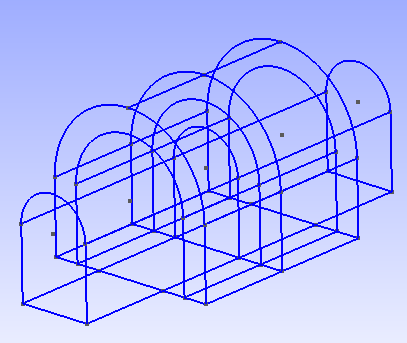
In the following, we will walk you through the entire process of creating a mesh for this geometry, including a number of common pitfalls by showing the things that can go wrong.
The first step in getting there was to create a coarse mesh, which was done by creating a 2d coarse mesh for each of cross sections, extruding them into the third direction, and gluing them together. The following code does this, using the techniques previously described:
This creates the following mesh:
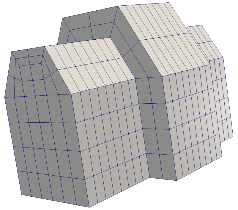
This mesh has the right general shape, but the top cells are now polygonal: their edges are no longer along circles and we do not have a very accurate representation of the original geometry. The next step is to teach the top part of the domain that it should be curved. Put another way, all calculations done on the top boundary cells should be done in cylindrical coordinates rather than Cartesian coordinates. We can do this by creating a CylindricalManifold object and associating it with the cells above y = 3. This way, when we refine the cells on top, we will place new points along concentric circles instead of straight lines.
In deal.II we describe all geometries with classes that inherit from Manifold. The default geometry is Cartesian and is implemented in the FlatManifold class. As the name suggests, Manifold and its inheriting classes provide a way to describe curves and curved cells in a general way with ideas and terminology from differential geometry: for example, CylindricalManifold inherits from ChartManifold, which describes a geometry through pull backs and push forwards. In general, one should think that the Triangulation class describes the topology of a domain (in addition, of course, to storing the locations of the vertices) while the Manifold classes describe the geometry of a domain (e.g., whether or not a pair of vertices lie along a circular arc or a straight line). A Triangulation will refine cells by doing computations with the Manifold associated with that cell regardless of whether or not the cell is on the boundary. Put another way: the Manifold classes do not need any information about where the boundary of the Triangulation actually is: it is up to the Triangulation to query the right Manifold for calculations on a cell. Most Manifold functions (e.g., Manifold::get_intermediate_point) know nothing about the domain itself and just assume that the points given to it lie along a geodesic. In this case, with the CylindricalManifold constructed below, the geodesics are arcs along circles orthogonal to the z-axis centered along the line (0, 3, z).
Since all three top parts of the domain use the same geodesics, we will mark all cells with centers above the y = 3 line as being cylindrical in nature:
With this code, we get a mesh that looks like this:
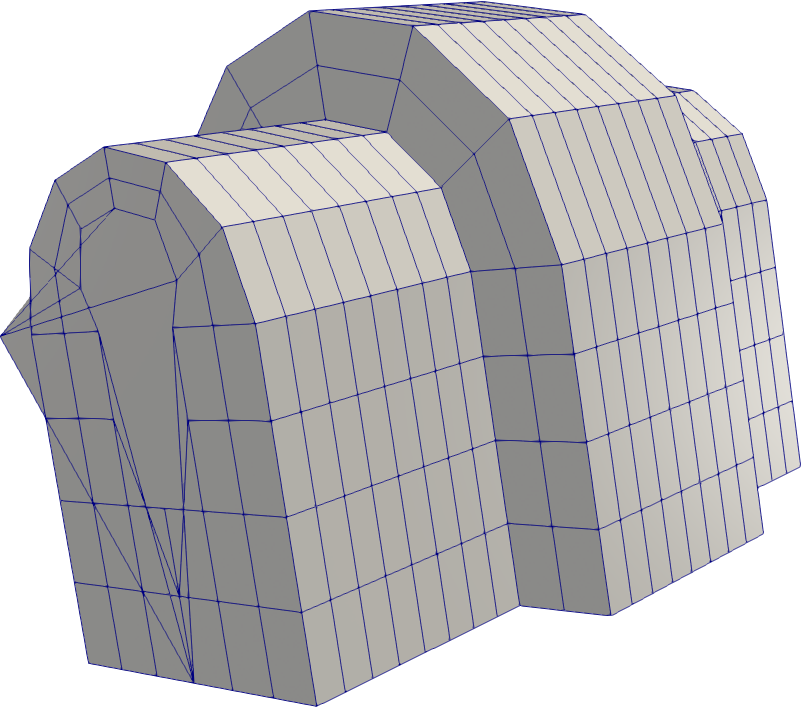
This change fixes the boundary but creates a new problem: the cells adjacent to the cylinder's axis are badly distorted. We should use Cartesian coordinates for calculations on these central cells to avoid this issue. The cells along the center line all have a face that touches the line (0, 3, z) so, to implement this, we go back and overwrite the manifold_ids on these cells to be zero (which is the default):
This gives us the following grid:
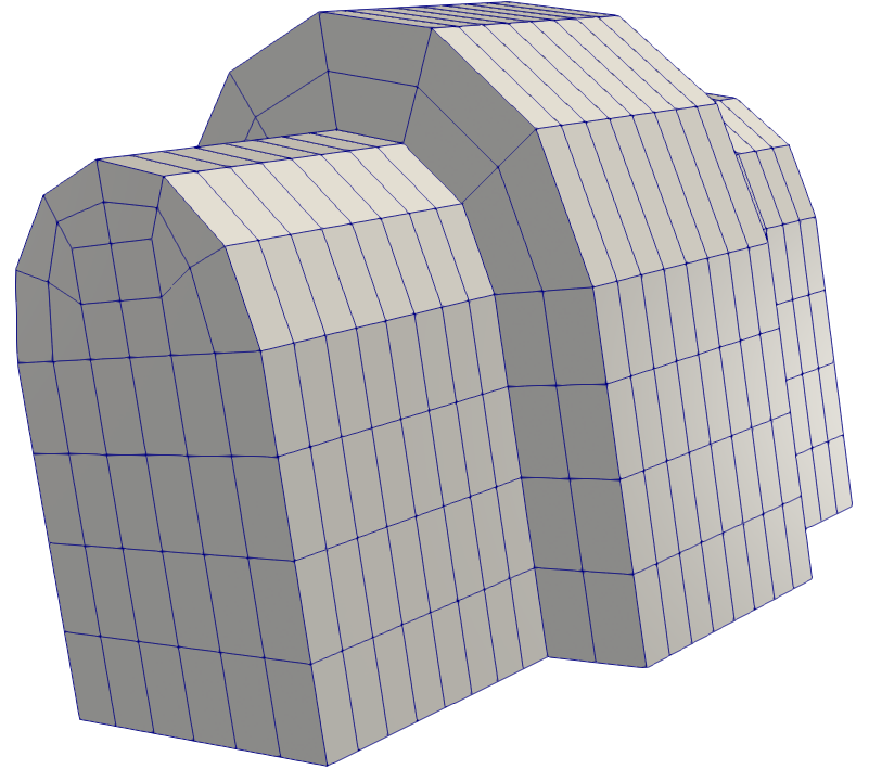
This gives us a good mesh, where cells at the center of each circle are still Cartesian and cells around the boundary lie along a circle. We can really see the nice detail of the boundary fitted mesh if we refine two more times:
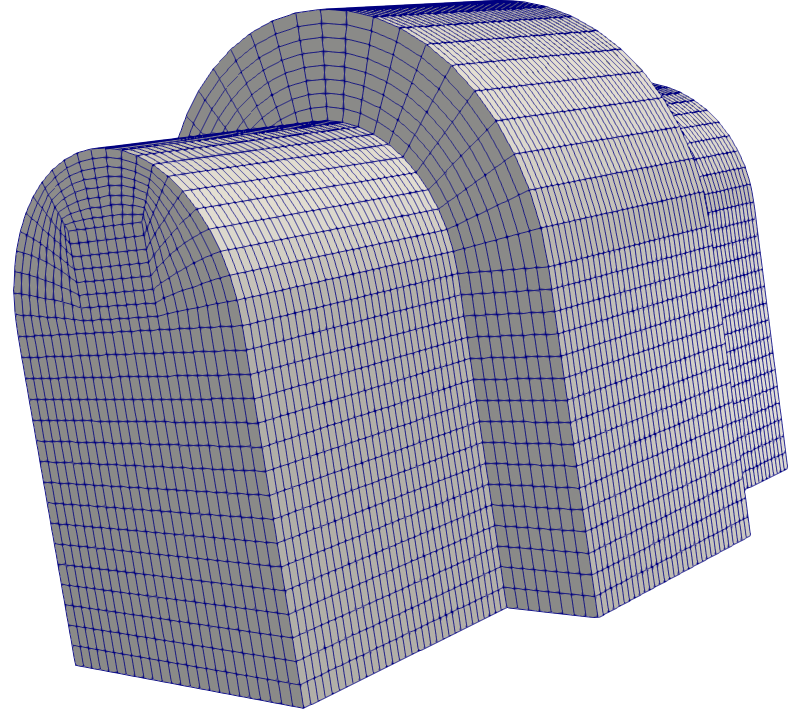
It is often useful to assign different boundary ids to a mesh that is generated in one form or another as described in this tutorial to apply different boundary conditions.
For example, you might want to apply a different boundary condition for the right boundary of the first grid in this program. To do this, iterate over the cells and their faces and identify the correct faces (for example using cell->center() to query the coordinates of the center of a cell as we do in step-1, or using cell->face(f)->get_boundary_id() to query the current boundary indicator of the fth face of the cell). You can then use cell->face(f)->set_boundary_id() to set the boundary id to something different. You can take a look back at step-1 how iteration over the meshes is done there.
Computations on manifolds, like they are done in step-38, require a surface mesh embedded into a higher dimensional space. While some can be constructed using the GridGenerator namespace or loaded from a file, it is sometimes useful to extract a surface mesh from a volume mesh.
Use the function GridGenerator::extract_boundary_mesh() to extract the surface elements of a mesh. Using the function on a 3d mesh (a Triangulation<3,3>, for example from grid_4()), this will return a Triangulation<2,3> that you can use in step-38. Also try extracting the boundary mesh of a Triangulation<2,2>.
 1.8.17