 |
Reference documentation for deal.II version 9.3.3
|
 |
Reference documentation for deal.II version 9.3.3
|
This tutorial depends on step-22.
This program was contributed by Martin Kronbichler and Wolfgang Bangerth.
This material is based upon work partly supported by the National Science Foundation under Award No. EAR-0426271 and The California Institute of Technology. Any opinions, findings, and conclusions or recommendations expressed in this publication are those of the author and do not necessarily reflect the views of the National Science Foundation or of The California Institute of Technology.
This program deals with an interesting physical problem: how does a fluid (i.e., a liquid or gas) behave if it experiences differences in buoyancy caused by temperature differences? It is clear that those parts of the fluid that are hotter (and therefore lighter) are going to rise up and those that are cooler (and denser) are going to sink down with gravity.
In cases where the fluid moves slowly enough such that inertial effects can be neglected, the equations that describe such behavior are the Boussinesq equations that read as follows:
\begin{eqnarray*} -\nabla \cdot (2 \eta \varepsilon ({\mathbf u})) + \nabla p &=& -\rho\; \beta \; T\; \mathbf{g}, \\ \nabla \cdot {\mathbf u} &=& 0, \\ \frac{\partial T}{\partial t} + {\mathbf u} \cdot \nabla T - \nabla \cdot \kappa \nabla T &=& \gamma. \end{eqnarray*}
These equations fall into the class of vector-valued problems (a toplevel overview of this topic can be found in the Handling vector valued problems module). Here, \mathbf u is the velocity field, p the pressure, and T the temperature of the fluid. \varepsilon ({\mathbf u}) = \frac 12 [(\nabla{\mathbf u}) + (\nabla {\mathbf u})^T] is the symmetric gradient of the velocity. As can be seen, velocity and pressure solve a Stokes equation describing the motion of an incompressible fluid, an equation we have previously considered in step-22; we will draw extensively on the experience we have gained in that program, in particular with regard to efficient linear Stokes solvers.
The forcing term of the fluid motion is the buoyancy of the fluid, expressed as the product of the density \rho, the thermal expansion coefficient \beta, the temperature T and the gravity vector \mathbf{g} pointing downward. (A derivation of why the right hand side looks like it looks is given in the introduction of step-32.) While the first two equations describe how the fluid reacts to temperature differences by moving around, the third equation states how the fluid motion affects the temperature field: it is an advection diffusion equation, i.e., the temperature is attached to the fluid particles and advected along in the flow field, with an additional diffusion (heat conduction) term. In many applications, the diffusion coefficient is fairly small, and the temperature equation is in fact transport, not diffusion dominated and therefore in character more hyperbolic than elliptic; we will have to take this into account when developing a stable discretization.
In the equations above, the term \gamma on the right hand side denotes the heat sources and may be a spatially and temporally varying function. \eta and \kappa denote the viscosity and diffusivity coefficients, which we assume constant for this tutorial program. The more general case when \eta depends on the temperature is an important factor in physical applications: Most materials become more fluid as they get hotter (i.e., \eta decreases with T); sometimes, as in the case of rock minerals at temperatures close to their melting point, \eta may change by orders of magnitude over the typical range of temperatures.
We note that the Stokes equation above could be nondimensionalized by introducing the Rayleigh number \mathrm{Ra}=\frac{\|\mathbf{g}\| \beta \rho}{\eta \kappa} \delta T L^3 using a typical length scale L, typical temperature difference \delta T, density \rho, thermal diffusivity \eta, and thermal conductivity \kappa. \mathrm{Ra} is a dimensionless number that describes the ratio of heat transport due to convection induced by buoyancy changes from temperature differences, and of heat transport due to thermal diffusion. A small Rayleigh number implies that buoyancy is not strong relative to viscosity and fluid motion \mathbf{u} is slow enough so that heat diffusion \kappa\nabla T is the dominant heat transport term. On the other hand, a fluid with a high Rayleigh number will show vigorous convection that dominates heat conduction.
For most fluids for which we are interested in computing thermal convection, the Rayleigh number is very large, often 10^6 or larger. From the structure of the equations, we see that this will lead to large pressure differences and large velocities. Consequently, the convection term in the convection-diffusion equation for T will also be very large and an accurate solution of this equation will require us to choose small time steps. Problems with large Rayleigh numbers are therefore hard to solve numerically for similar reasons that make solving the Navier-Stokes equations hard to solve when the Reynolds number \mathrm{Re} is large.
Note that a large Rayleigh number does not necessarily involve large velocities in absolute terms. For example, the Rayleigh number in the earth mantle is larger than 10^6. Yet the velocities are small: the material is in fact solid rock but it is so hot and under pressure that it can flow very slowly, on the order of at most a few centimeters per year. Nevertheless, this can lead to mixing over time scales of many million years, a time scale much shorter than for the same amount of heat to be distributed by thermal conductivity and a time scale of relevance to affect the evolution of the earth's interior and surface structure.
Since the Boussinesq equations are derived under the assumption that inertia of the fluid's motion does not play a role, the flow field is at each time entirely determined by buoyancy difference at that time, not by the flow field at previous times. This is reflected by the fact that the first two equations above are the steady state Stokes equation that do not contain a time derivative. Consequently, we do not need initial conditions for either velocities or pressure. On the other hand, the temperature field does satisfy an equation with a time derivative, so we need initial conditions for T.
As for boundary conditions: if \kappa>0 then the temperature satisfies a second order differential equation that requires boundary data all around the boundary for all times. These can either be a prescribed boundary temperature T|_{\partial\Omega}=T_b (Dirichlet boundary conditions), or a prescribed thermal flux \mathbf{n}\cdot\kappa\nabla T|_{\partial\Omega}=\phi; in this program, we will use an insulated boundary condition, i.e., prescribe no thermal flux: \phi=0.
Similarly, the velocity field requires us to pose boundary conditions. These may be no-slip no-flux conditions \mathbf{u}=0 on \partial\Omega if the fluid sticks to the boundary, or no normal flux conditions \mathbf n \cdot \mathbf u = 0 if the fluid can flow along but not across the boundary, or any number of other conditions that are physically reasonable. In this program, we will use no normal flux conditions.
Like the equations solved in step-21, we here have a system of differential-algebraic equations (DAE): with respect to the time variable, only the temperature equation is a differential equation whereas the Stokes system for \mathbf{u} and p has no time-derivatives and is therefore of the sort of an algebraic constraint that has to hold at each time instant. The main difference to step-21 is that the algebraic constraint there was a mixed Laplace system of the form
\begin{eqnarray*} \mathbf u + {\mathbf K}\lambda \nabla p &=& 0, \\ \nabla\cdot \mathbf u &=& f, \end{eqnarray*}
where now we have a Stokes system
\begin{eqnarray*} -\nabla \cdot (2 \eta \varepsilon ({\mathbf u})) + \nabla p &=& f, \\ \nabla\cdot \mathbf u &=& 0, \end{eqnarray*}
where \nabla \cdot \eta \varepsilon (\cdot) is an operator similar to the Laplacian \Delta applied to a vector field.
Given the similarity to what we have done in step-21, it may not come as a surprise that we choose a similar approach, although we will have to make adjustments for the change in operator in the top-left corner of the differential operator.
The structure of the problem as a DAE allows us to use the same strategy as we have already used in step-21, i.e., we use a time lag scheme: we first solve the temperature equation (using an extrapolated velocity field), and then insert the new temperature solution into the right hand side of the velocity equation. The way we implement this in our code looks at things from a slightly different perspective, though. We first solve the Stokes equations for velocity and pressure using the temperature field from the previous time step, which means that we get the velocity for the previous time step. In other words, we first solve the Stokes system for time step n - 1 as
\begin{eqnarray*} -\nabla \cdot (2\eta \varepsilon ({\mathbf u}^{n-1})) + \nabla p^{n-1} &=& -\rho\; \beta \; T^{n-1} \mathbf{g}, \\ \nabla \cdot {\mathbf u}^{n-1} &=& 0, \end{eqnarray*}
and then the temperature equation with an extrapolated velocity field to time n.
In contrast to step-21, we'll use a higher order time stepping scheme here, namely the Backward Differentiation Formula scheme of order 2 (BDF-2 in short) that replaces the time derivative \frac{\partial T}{\partial t} by the (one-sided) difference quotient \frac{\frac 32 T^{n}-2T^{n-1}+\frac 12 T^{n-2}}{k} with k the time step size. This gives the discretized-in-time temperature equation
\begin{eqnarray*} \frac 32 T^n - k\nabla \cdot \kappa \nabla T^n &=& 2 T^{n-1} - \frac 12 T^{n-2} - k(2{\mathbf u}^{n-1} - {\mathbf u}^{n-2} ) \cdot \nabla (2T^{n-1}-T^{n-2}) + k\gamma. \end{eqnarray*}
Note how the temperature equation is solved semi-explicitly: diffusion is treated implicitly whereas advection is treated explicitly using an extrapolation (or forward-projection) of temperature and velocity, including the just-computed velocity {\mathbf u}^{n-1}. The forward-projection to the current time level n is derived from a Taylor expansion, T^n \approx T^{n-1} + k_n \frac{\partial T}{\partial t} \approx T^{n-1} + k_n \frac{T^{n-1}-T^{n-2}}{k_n} = 2T^{n-1}-T^{n-2}. We need this projection for maintaining the order of accuracy of the BDF-2 scheme. In other words, the temperature fields we use in the explicit right hand side are second order approximations of the current temperature field — not quite an explicit time stepping scheme, but by character not too far away either.
The introduction of the temperature extrapolation limits the time step by a Courant-Friedrichs-Lewy (CFL) condition just like it was in step-21. (We wouldn't have had that stability condition if we treated the advection term implicitly since the BDF-2 scheme is A-stable, at the price that we needed to build a new temperature matrix at each time step.) We will discuss the exact choice of time step in the results section, but for the moment of importance is that this CFL condition means that the time step size k may change from time step to time step, and that we have to modify the above formula slightly. If k_n,k_{n-1} are the time steps sizes of the current and previous time step, then we use the approximations
\begin{align*} \frac{\partial T}{\partial t} \approx \frac 1{k_n} \left( \frac{2k_n+k_{n-1}}{k_n+k_{n-1}} T^{n} - \frac{k_n+k_{n-1}}{k_{n-1}}T^{n-1} + \frac{k_n^2}{k_{n-1}(k_n+k_{n-1})} T^{n-2} \right) \end{align*}
and
\begin{align*} T^n \approx T^{n-1} + k_n \frac{\partial T}{\partial t} \approx T^{n-1} + k_n \frac{T^{n-1}-T^{n-2}}{k_{n-1}} = \left(1+\frac{k_n}{k_{n-1}}\right)T^{n-1}-\frac{k_n}{k_{n-1}}T^{n-2}, \end{align*}
and above equation is generalized as follows:
\begin{eqnarray*} \frac{2k_n+k_{n-1}}{k_n+k_{n-1}} T^n - k_n\nabla \cdot \kappa \nabla T^n &=& \frac{k_n+k_{n-1}}{k_{n-1}} T^{n-1} - \frac{k_n^2}{k_{n-1}(k_n+k_{n-1})} T^{n-2} - k_n{\mathbf u}^{*,n} \cdot \nabla T^{*,n} + k_n\gamma, \end{eqnarray*}
where {(\cdot)}^{*,n} = \left(1+\frac{k_n}{k_{n-1}}\right)(\cdot)^{n-1} - \frac{k_n}{k_{n-1}}(\cdot)^{n-2} denotes the extrapolation of velocity \mathbf u and temperature T to time level n, using the values at the two previous time steps. That's not an easy to read equation, but will provide us with the desired higher order accuracy. As a consistency check, it is easy to verify that it reduces to the same equation as above if k_n=k_{n-1}.
As a final remark we note that the choice of a higher order time stepping scheme of course forces us to keep more time steps in memory; in particular, we here will need to have T^{n-2} around, a vector that we could previously discard. This seems like a nuisance that we were able to avoid previously by using only a first order time stepping scheme, but as we will see below when discussing the topic of stabilization, we will need this vector anyway and so keeping it around for time discretization is essentially for free and gives us the opportunity to use a higher order scheme.
Like solving the mixed Laplace equations, solving the Stokes equations requires us to choose particular pairs of finite elements for velocities and pressure variables. Because this has already been discussed in step-22, we only cover this topic briefly: Here, we use the stable pair Q_{p+1}^d \times Q_p, p\ge 1. These are continuous elements, so we can form the weak form of the Stokes equation without problem by integrating by parts and substituting continuous functions by their discrete counterparts:
\begin{eqnarray*} (\nabla {\mathbf v}_h, 2\eta \varepsilon ({\mathbf u}^{n-1}_h)) - (\nabla \cdot {\mathbf v}_h, p^{n-1}_h) &=& -({\mathbf v}_h, \rho\; \beta \; T^{n-1}_h \mathbf{g}), \\ (q_h, \nabla \cdot {\mathbf u}^{n-1}_h) &=& 0, \end{eqnarray*}
for all test functions \mathbf v_h, q_h. The first term of the first equation is considered as the inner product between tensors, i.e. (\nabla {\mathbf v}_h, \eta \varepsilon ({\mathbf u}^{n-1}_h))_\Omega = \int_\Omega \sum_{i,j=1}^d [\nabla {\mathbf v}_h]_{ij} \eta [\varepsilon ({\mathbf u}^{n-1}_h)]_{ij}\, dx. Because the second tensor in this product is symmetric, the anti-symmetric component of \nabla {\mathbf v}_h plays no role and it leads to the entirely same form if we use the symmetric gradient of \mathbf v_h instead. Consequently, the formulation we consider and that we implement is
\begin{eqnarray*} (\varepsilon({\mathbf v}_h), 2\eta \varepsilon ({\mathbf u}^{n-1}_h)) - (\nabla \cdot {\mathbf v}_h, p^{n-1}_h) &=& -({\mathbf v}_h, \rho\; \beta \; T^{n-1}_h \mathbf{g}), \\ (q_h, \nabla \cdot {\mathbf u}^{n-1}_h) &=& 0. \end{eqnarray*}
This is exactly the same as what we already discussed in step-22 and there is not much more to say about this here.
The more interesting question is what to do with the temperature advection-diffusion equation. By default, not all discretizations of this equation are equally stable unless we either do something like upwinding, stabilization, or all of this. One way to achieve this is to use discontinuous elements (i.e., the FE_DGQ class that we used, for example, in the discretization of the transport equation in step-12, or in discretizing the pressure in step-20 and step-21) and to define a flux at the interface between cells that takes into account upwinding. If we had a pure advection problem this would probably be the simplest way to go. However, here we have some diffusion as well, and the discretization of the Laplace operator with discontinuous elements is cumbersome because of the significant number of additional terms that need to be integrated on each face between cells. Discontinuous elements also have the drawback that the use of numerical fluxes introduces an additional numerical diffusion that acts everywhere, whereas we would really like to minimize the effect of numerical diffusion to a minimum and only apply it where it is necessary to stabilize the scheme.
A better alternative is therefore to add some nonlinear viscosity to the model. Essentially, what this does is to transform the temperature equation from the form
\begin{eqnarray*} \frac{\partial T}{\partial t} + {\mathbf u} \cdot \nabla T - \nabla \cdot \kappa \nabla T &=& \gamma \end{eqnarray*}
to something like
\begin{eqnarray*} \frac{\partial T}{\partial t} + {\mathbf u} \cdot \nabla T - \nabla \cdot (\kappa+\nu(T)) \nabla T &=& \gamma, \end{eqnarray*}
where \nu(T) is an addition viscosity (diffusion) term that only acts in the vicinity of shocks and other discontinuities. \nu(T) is chosen in such a way that if T satisfies the original equations, the additional viscosity is zero.
To achieve this, the literature contains a number of approaches. We will here follow one developed by Guermond and Popov that builds on a suitably defined residual and a limiting procedure for the additional viscosity. To this end, let us define a residual R_\alpha(T) as follows:
\begin{eqnarray*} R_\alpha(T) = \left( \frac{\partial T}{\partial t} + {\mathbf u} \cdot \nabla T - \nabla \cdot \kappa \nabla T - \gamma \right) T^{\alpha-1} \end{eqnarray*}
where we will later choose the stabilization exponent \alpha from within the range [1,2]. Note that R_\alpha(T) will be zero if T satisfies the temperature equation, since then the term in parentheses will be zero. Multiplying terms out, we get the following, entirely equivalent form:
\begin{eqnarray*} R_\alpha(T) = \frac 1\alpha \frac{\partial (T^\alpha)}{\partial t} + \frac 1\alpha {\mathbf u} \cdot \nabla (T^\alpha) - \frac 1\alpha \nabla \cdot \kappa \nabla (T^\alpha) + \kappa(\alpha-1) T^{\alpha-2} |\nabla T|^2 - \gamma T^{\alpha-1} \end{eqnarray*}
With this residual, we can now define the artificial viscosity as a piecewise constant function defined on each cell K with diameter h_K separately as follows:
\begin{eqnarray*} \nu_\alpha(T)|_K = \beta \|\mathbf{u}\|_{L^\infty(K)} \min\left\{ h_K, h_K^\alpha \frac{\|R_\alpha(T)\|_{L^\infty(K)}}{c(\mathbf{u},T)} \right\} \end{eqnarray*}
Here, \beta is a stabilization constant (a dimensional analysis reveals that it is unitless and therefore independent of scaling; we will discuss its choice in the results section) and c(\mathbf{u},T) is a normalization constant that must have units \frac{m^{\alpha-1}K^\alpha}{s}. We will choose it as c(\mathbf{u},T) = c_R\ \|\mathbf{u}\|_{L^\infty(\Omega)} \ \mathrm{var}(T) \ |\mathrm{diam}(\Omega)|^{\alpha-2}, where \mathrm{var}(T)=\max_\Omega T - \min_\Omega T is the range of present temperature values (remember that buoyancy is driven by temperature variations, not the absolute temperature) and c_R is a dimensionless constant. To understand why this method works consider this: If on a particular cell K the temperature field is smooth, then we expect the residual to be small there (in fact to be on the order of {\cal O}(h_K)) and the stabilization term that injects artificial diffusion will there be of size h_K^{\alpha+1} — i.e., rather small, just as we hope it to be when no additional diffusion is necessary. On the other hand, if we are on or close to a discontinuity of the temperature field, then the residual will be large; the minimum operation in the definition of \nu_\alpha(T) will then ensure that the stabilization has size h_K — the optimal amount of artificial viscosity to ensure stability of the scheme.
Whether or not this scheme really works is a good question. Computations by Guermond and Popov have shown that this form of stabilization actually performs much better than most of the other stabilization schemes that are around (for example streamline diffusion, to name only the simplest one). Furthermore, for \alpha\in [1,2) they can even prove that it produces better convergence orders for the linear transport equation than for example streamline diffusion. For \alpha=2, no theoretical results are currently available, but numerical tests indicate that the results are considerably better than for \alpha=1.
A more practical question is how to introduce this artificial diffusion into the equations we would like to solve. Note that the numerical viscosity \nu(T) is temperature-dependent, so the equation we want to solve is nonlinear in T — not what one desires from a simple method to stabilize an equation, and even less so if we realize that \nu(T) is nondifferentiable in T. However, there is no reason to despair: we still have to discretize in time and we can treat the term explicitly.
In the definition of the stabilization parameter, we approximate the time derivative by \frac{\partial T}{\partial t} \approx \frac{T^{n-1}-T^{n-2}}{k^{n-1}}. This approximation makes only use of available time data and this is the reason why we need to store data of two previous time steps (which enabled us to use the BDF-2 scheme without additional storage cost). We could now simply evaluate the rest of the terms at t_{n-1}, but then the discrete residual would be nothing else than a backward Euler approximation, which is only first order accurate. So, in case of smooth solutions, the residual would be still of the order h, despite the second order time accuracy in the outer BDF-2 scheme and the spatial FE discretization. This is certainly not what we want to have (in fact, we desired to have small residuals in regions where the solution behaves nicely), so a bit more care is needed. The key to this problem is to observe that the first derivative as we constructed it is actually centered at t_{n-\frac{3}{2}}. We get the desired second order accurate residual calculation if we evaluate all spatial terms at t_{n-\frac{3}{2}} by using the approximation \frac 12 T^{n-1}+\frac 12 T^{n-2}, which means that we calculate the nonlinear viscosity as a function of this intermediate temperature, \nu_\alpha = \nu_\alpha\left(\frac 12 T^{n-1}+\frac 12 T^{n-2}\right). Note that this evaluation of the residual is nothing else than a Crank-Nicholson scheme, so we can be sure that now everything is alright. One might wonder whether it is a problem that the numerical viscosity now is not evaluated at time n (as opposed to the rest of the equation). However, this offset is uncritical: For smooth solutions, \nu_\alpha will vary continuously, so the error in time offset is k times smaller than the nonlinear viscosity itself, i.e., it is a small higher order contribution that is left out. That's fine because the term itself is already at the level of discretization error in smooth regions.
Using the BDF-2 scheme introduced above, this yields for the simpler case of uniform time steps of size k:
\begin{eqnarray*} \frac 32 T^n - k\nabla \cdot \kappa \nabla T^n &=& 2 T^{n-1} - \frac 12 T^{n-2} \\ && + k\nabla \cdot \left[ \nu_\alpha\left(\frac 12 T^{n-1}+\frac 12 T^{n-2}\right) \ \nabla (2T^{n-1}-T^{n-2}) \right] \\ && - k(2{\mathbf u}^{n-1}-{\mathbf u}^{n-2}) \cdot \nabla (2T^{n-1}-T^{n-2}) \\ && + k\gamma. \end{eqnarray*}
On the left side of this equation remains the term from the time derivative and the original (physical) diffusion which we treat implicitly (this is actually a nice term: the matrices that result from the left hand side are the mass matrix and a multiple of the Laplace matrix — both are positive definite and if the time step size k is small, the sum is simple to invert). On the right hand side, the terms in the first line result from the time derivative; in the second line is the artificial diffusion at time t_{n-\frac 32}; the third line contains the advection term, and the fourth the sources. Note that the artificial diffusion operates on the extrapolated temperature at the current time in the same way as we have discussed the advection works in the section on time stepping.
The form for nonuniform time steps that we will have to use in reality is a bit more complicated (which is why we showed the simpler form above first) and reads:
\begin{eqnarray*} \frac{2k_n+k_{n-1}}{k_n+k_{n-1}} T^n - k_n\nabla \cdot \kappa \nabla T^n &=& \frac{k_n+k_{n-1}}{k_{n-1}} T^{n-1} - \frac{k_n^2}{k_{n-1}(k_n+k_{n-1})} T^{n-2} \\ && + k_n\nabla \cdot \left[ \nu_\alpha\left(\frac 12 T^{n-1}+\frac 12 T^{n-2}\right) \ \nabla \left[ \left(1+\frac{k_n}{k_{n-1}}\right)T^{n-1}-\frac{k_n}{k_{n-1}}T^{n-2} \right] \right] \\ && - k_n \left[ \left(1+\frac{k_n}{k_{n-1}}\right){\mathbf u}^{n-1} - \frac{k_n}{k_{n-1}}{\mathbf u}^{n-2} \right] \cdot \nabla \left[ \left(1+\frac{k_n}{k_{n-1}}\right)T^{n-1}-\frac{k_n}{k_{n-1}}T^{n-2} \right] \\ && + k_n\gamma. \end{eqnarray*}
After settling all these issues, the weak form follows naturally from the strong form shown in the last equation, and we immediately arrive at the weak form of the discretized equations:
\begin{eqnarray*} \frac{2k_n+k_{n-1}}{k_n+k_{n-1}} (\tau_h,T_h^n) + k_n (\nabla \tau_h, \kappa \nabla T_h^n) &=& \biggl(\tau_h, \frac{k_n+k_{n-1}}{k_{n-1}} T_h^{n-1} - \frac{k_n^2}{k_{n-1}(k_n+k_{n-1})} T_h^{n-2} \\ &&\qquad - k_n \left[ \left(1+\frac{k_n}{k_{n-1}}\right){\mathbf u}^{n-1} - \frac{k_n}{k_{n-1}}{\mathbf u}^{n-2} \right] \cdot \nabla \left[ \left(1+\frac{k_n}{k_{n-1}}\right)T^{n-1}-\frac{k_n}{k_{n-1}}T^{n-2} \right] + k_n\gamma \biggr) \\ && - k_n \left(\nabla \tau_h, \nu_\alpha\left(\frac 12 T_h^{n-1}+\frac 12 T_h^{n-2}\right) \ \nabla \left[ \left(1+\frac{k_n}{k_{n-1}}\right)T^{n-1}-\frac{k_n}{k_{n-1}}T^{n-2} \right] \right) \end{eqnarray*}
for all discrete test functions \tau_h. Here, the diffusion term has been integrated by parts, and we have used that we will impose no thermal flux, \mathbf{n}\cdot\kappa\nabla T|_{\partial\Omega}=0.
This then results in a matrix equation of form
\begin{eqnarray*} \left( \frac{2k_n+k_{n-1}}{k_n+k_{n-1}} M+k_n A_T\right) T_h^n = F(U_h^{n-1}, U_h^{n-2},T_h^{n-1},T_h^{n-2}), \end{eqnarray*}
which given the structure of matrix on the left (the sum of two positive definite matrices) is easily solved using the Conjugate Gradient method.
As explained above, our approach to solving the joint system for velocities/pressure on the one hand and temperature on the other is to use an operator splitting where we first solve the Stokes system for the velocities and pressures using the old temperature field, and then solve for the new temperature field using the just computed velocity field. (A more extensive discussion of operator splitting methods can be found in step-58.)
Solving the linear equations coming from the Stokes system has been discussed in great detail in step-22. In particular, in the results section of that program, we have discussed a number of alternative linear solver strategies that turned out to be more efficient than the original approach. The best alternative identified there we to use a GMRES solver preconditioned by a block matrix involving the Schur complement. Specifically, the Stokes operator leads to a block structured matrix
\begin{eqnarray*} \left(\begin{array}{cc} A & B^T \\ B & 0 \end{array}\right) \end{eqnarray*}
and as discussed there a good preconditioner is
\begin{eqnarray*} P = \left(\begin{array}{cc} A & 0 \\ B & -S \end{array}\right), \qquad \text{or equivalently} \qquad P^{-1} = \left(\begin{array}{cc} A^{-1} & 0 \\ S^{-1} B A^{-1} & -S^{-1} \end{array}\right) \end{eqnarray*}
where S is the Schur complement of the Stokes operator S=B^TA^{-1}B. Of course, this preconditioner is not useful because we can't form the various inverses of matrices, but we can use the following as a preconditioner:
\begin{eqnarray*} \tilde P^{-1} = \left(\begin{array}{cc} \tilde A^{-1} & 0 \\ \tilde S^{-1} B \tilde A^{-1} & -\tilde S^{-1} \end{array}\right) \end{eqnarray*}
where \tilde A^{-1},\tilde S^{-1} are approximations to the inverse matrices. In particular, it turned out that S is spectrally equivalent to the mass matrix and consequently replacing \tilde S^{-1} by a CG solver applied to the mass matrix on the pressure space was a good choice. In a small deviation from step-22, we here have a coefficient \eta in the momentum equation, and by the same derivation as there we should arrive at the conclusion that it is the weighted mass matrix with entries \tilde S_{ij}=(\eta^{-1}\varphi_i,\varphi_j) that we should be using.
It was more complicated to come up with a good replacement \tilde A^{-1}, which corresponds to the discretized symmetric Laplacian of the vector-valued velocity field, i.e. A_{ij} = (\varepsilon {\mathbf v}_i, 2\eta \varepsilon ({\mathbf v}_j)). In step-22 we used a sparse LU decomposition (using the SparseDirectUMFPACK class) of A for \tilde A^{-1} — the perfect preconditioner — in 2d, but for 3d memory and compute time is not usually sufficient to actually compute this decomposition; consequently, we only use an incomplete LU decomposition (ILU, using the SparseILU class) in 3d.
For this program, we would like to go a bit further. To this end, note that the symmetrized bilinear form on vector fields, (\varepsilon {\mathbf v}_i, 2 \eta \varepsilon ({\mathbf v}_j)) is not too far away from the nonsymmetrized version, (\nabla {\mathbf v}_i, \eta \nabla {\mathbf v}_j)
= \sum_{k,l=1}^d
(\partial_k ({\mathbf v}_i)_l, \eta \partial_k ({\mathbf v}_j)_l)
(note that the factor 2 has disappeared in this form). The latter, however, has the advantage that the dim vector components of the test functions are not coupled (well, almost, see below), i.e., the resulting matrix is block-diagonal: one block for each vector component, and each of these blocks is equal to the Laplace matrix for this vector component. So assuming we order degrees of freedom in such a way that first all x-components of the velocity are numbered, then the y-components, and then the z-components, then the matrix \hat A that is associated with this slightly different bilinear form has the form
\begin{eqnarray*} \hat A = \left(\begin{array}{ccc} A_s & 0 & 0 \\ 0 & A_s & 0 \\ 0 & 0 & A_s \end{array}\right) \end{eqnarray*}
where A_s is a Laplace matrix of size equal to the number of shape functions associated with each component of the vector-valued velocity. With this matrix, one could be tempted to define our preconditioner for the velocity matrix A as follows:
\begin{eqnarray*} \tilde A^{-1} = \left(\begin{array}{ccc} \tilde A_s^{-1} & 0 & 0 \\ 0 & \tilde A_s^{-1} & 0 \\ 0 & 0 & \tilde A_s^{-1} \end{array}\right), \end{eqnarray*}
where \tilde A_s^{-1} is a preconditioner for the Laplace matrix — something where we know very well how to build good preconditioners!
In reality, the story is not quite as simple: To make the matrix \tilde A definite, we need to make the individual blocks \tilde A_s definite by applying boundary conditions. One can try to do so by applying Dirichlet boundary conditions all around the boundary, and then the so-defined preconditioner \tilde A^{-1} turns out to be a good preconditioner for A if the latter matrix results from a Stokes problem where we also have Dirichlet boundary conditions on the velocity components all around the domain, i.e., if we enforce \mathbf{u} = 0.
Unfortunately, this "if" is an "if and only if": in the program below we will want to use no-flux boundary conditions of the form \mathbf u \cdot \mathbf n = 0 (i.e., flow parallel to the boundary is allowed, but no flux through the boundary). In this case, it turns out that the block diagonal matrix defined above is not a good preconditioner because it neglects the coupling of components at the boundary. A better way to do things is therefore if we build the matrix \hat A as the vector Laplace matrix \hat A_{ij} = (\nabla {\mathbf v}_i, \eta \nabla {\mathbf v}_j) and then apply the same boundary condition as we applied to A. If this is a Dirichlet boundary condition all around the domain, the \hat A will decouple to three diagonal blocks as above, and if the boundary conditions are of the form \mathbf u \cdot \mathbf n = 0 then this will introduce a coupling of degrees of freedom at the boundary but only there. This, in fact, turns out to be a much better preconditioner than the one introduced above, and has almost all the benefits of what we hoped to get.
To sum this whole story up, we can observe:
Compared to building a preconditioner from the original matrix A resulting from the symmetric gradient as we did in step-22, we have to expect that the preconditioner based on the Laplace bilinear form performs worse since it does not take into account the coupling between vector components.
On the other hand, preconditioners for the Laplace matrix are typically more mature and perform better than ones for vector problems. For example, at the time of this writing, Algebraic Multigrid (AMG) algorithms are very well developed for scalar problems, but not so for vector problems.
This is the easy part: The matrix for the temperature equation has the form \alpha M + \beta A, where M,A are mass and stiffness matrices on the temperature space, and \alpha,\beta are constants related the time stepping scheme and the current and previous time step. This being the sum of a symmetric positive definite and a symmetric positive semidefinite matrix, the result is also symmetric positive definite. Furthermore, \frac\beta\alpha is a number proportional to the time step, and so becomes small whenever the mesh is fine, damping the effect of the then ill-conditioned stiffness matrix.
As a consequence, inverting this matrix with the Conjugate Gradient algorithm, using a simple preconditioner, is trivial and very cheap compared to inverting the Stokes matrix.
One of the things worth explaining up front about the program below is the use of two different DoFHandler objects. If one looks at the structure of the equations above and the scheme for their solution, one realizes that there is little commonality that keeps the Stokes part and the temperature part together. In all previous tutorial programs in which we have discussed vector-valued problems we have always only used a single finite element with several vector components, and a single DoFHandler object. Sometimes, we have substructured the resulting matrix into blocks to facilitate particular solver schemes; this was, for example, the case in the step-22 program for the Stokes equations upon which the current program is based.
We could of course do the same here. The linear system that we would get would look like this:
\begin{eqnarray*} \left(\begin{array}{ccc} A & B^T & 0 \\ B & 0 &0 \\ C & 0 & K \end{array}\right) \left(\begin{array}{ccc} U^{n-1} \\ P^{n-1} \\ T^n \end{array}\right) = \left(\begin{array}{ccc} F_U(T^{n-1}) \\ 0 \\ F_T(U^{n-1},U^{n-2},T^{n-1},T^{n-2}) \end{array}\right). \end{eqnarray*}
The problem with this is: We never use the whole matrix at the same time. In fact, it never really exists at the same time: As explained above, K and F_T depend on the already computed solution U^n, in the first case through the time step (that depends on U^n because it has to satisfy a CFL condition). So we can only assemble it once we've already solved the top left 2\times 2 block Stokes system, and once we've moved on to the temperature equation we don't need the Stokes part any more; the fact that we build an object for a matrix that never exists as a whole in memory at any given time led us to jumping through some hoops in step-21, so let's not repeat this sort of error. Furthermore, we don't actually build the matrix C: Because by the time we get to the temperature equation we already know U^n, and because we have to assemble the right hand side F_T at this time anyway, we simply move the term CU^n to the right hand side and assemble it along with all the other terms there. What this means is that there does not remain a part of the matrix where temperature variables and Stokes variables couple, and so a global enumeration of all degrees of freedom is no longer important: It is enough if we have an enumeration of all Stokes degrees of freedom, and of all temperature degrees of freedom independently.
In essence, there is consequently not much use in putting everything into a block matrix (though there are of course the same good reasons to do so for the 2\times 2 Stokes part), or, for that matter, in putting everything into the same DoFHandler object.
But are there downsides to doing so? These exist, though they may not be obvious at first. The main problem is that if we need to create one global finite element that contains velocity, pressure, and temperature shape functions, and use this to initialize the DoFHandler. But we also use this finite element object to initialize all FEValues or FEFaceValues objects that we use. This may not appear to be that big a deal, but imagine what happens when, for example, we evaluate the residual
R_\alpha(T)
=
\left(
\frac{\partial T}{\partial t}
+
{\mathbf u} \cdot \nabla T
-
\nabla \cdot \kappa \nabla T - \gamma
\right)
T^{\alpha-1}
that we need to compute the artificial viscosity \nu_\alpha(T)|_K. For this, we need the Laplacian of the temperature, which we compute using the tensor of second derivatives (Hessians) of the shape functions (we have to give the update_hessians flag to the FEValues object for this). Now, if we have a finite that contains the shape functions for velocities, pressures, and temperatures, that means that we have to compute the Hessians of all shape functions, including the many higher order shape functions for the velocities. That's a lot of computations that we don't need, and indeed if one were to do that (as we had in an early version of the program), assembling the right hand side took about a quarter of the overall compute time.
So what we will do is to use two different finite element objects, one for the Stokes components and one for the temperatures. With this come two different DoFHandlers, two sparsity patterns and two matrices for the Stokes and temperature parts, etc. And whenever we have to assemble something that contains both temperature and Stokes shape functions (in particular the right hand sides of Stokes and temperature equations), then we use two FEValues objects initialized with two cell iterators that we walk in parallel through the two DoFHandler objects associated with the same Triangulation object; for these two FEValues objects, we use of course the same quadrature objects so that we can iterate over the same set of quadrature points, but each FEValues object will get update flags only according to what it actually needs to compute. In particular, when we compute the residual as above, we only ask for the values of the Stokes shape functions, but also the Hessians of the temperature shape functions — much cheaper indeed, and as it turns out: assembling the right hand side of the temperature equation is now a component of the program that is hardly measurable.
With these changes, timing the program yields that only the following operations are relevant for the overall run time:
BoussinesqFlowProblem::setup_dofs: 7% of overall run time. In essence this means that all bottlenecks apart from the algebraic multigrid have been removed.
In much the same way as we used PETSc to support our linear algebra needs in step-17 and step-18, we use interfaces to the Trilinos library (see the deal.II README file for installation instructions) in this program. Trilinos is a very large collection of everything that has to do with linear and nonlinear algebra, as well as all sorts of tools around that (and looks like it will grow in many other directions in the future as well).
The main reason for using Trilinos, similar to our exploring PETSc, is that it is a very powerful library that provides a lot more tools than deal.II's own linear algebra library. That includes, in particular, the ability to work in parallel on a cluster, using MPI, and a wider variety of preconditioners. In the latter class, one of the most interesting capabilities is the existence of the Trilinos ML package that implements an Algebraic Multigrid (AMG) method. We will use this preconditioner to precondition the second order operator part of the momentum equation. The ability to solve problems in parallel will be explored in step-32, using the same problem as discussed here.
PETSc, which we have used in step-17 and step-18, is certainly a powerful library, providing a large number of functions that deal with matrices, vectors, and iterative solvers and preconditioners, along with lots of other stuff, most of which runs quite well in parallel. It is, however, a few years old already than Trilinos, written in C, and generally not quite as easy to use as some other libraries. As a consequence, deal.II has also acquired interfaces to Trilinos, which shares a lot of the same functionality with PETSc. It is, however, a project that is several years younger, is written in C++ and by people who generally have put a significant emphasis on software design.
The case we want to solve here is as follows: we solve the Boussinesq equations described above with \kappa=10^{-6}, \eta=1, \rho=1, \beta=10, i.e., a relatively slow moving fluid that has virtually no thermal diffusive conductivity and transports heat mainly through convection. On the boundary, we will require no-normal flux for the velocity ( \mathrm{n}\cdot\mathrm{u}=0) and for the temperature ( \mathrm{n}\cdot\nabla T=0). This is one of the cases discussed in the introduction of step-22 and fixes one component of the velocity while allowing flow to be parallel to the boundary. There remain dim-1 components to be fixed, namely the tangential components of the normal stress; for these, we choose homogeneous conditions which means that we do not have to anything special. Initial conditions are only necessary for the temperature field, and we choose it to be constant zero.
The evolution of the problem is then entirely driven by the right hand side \gamma(\mathrm{x},t) of the temperature equation, i.e., by heat sources and sinks. Here, we choose a setup invented in advance of a Christmas lecture: real candles are of course prohibited in U.S. class rooms, but virtual ones are allowed. We therefore choose three spherical heat sources unequally spaced close to the bottom of the domain, imitating three candles. The fluid located at these sources, initially at rest, is then heated up and as the temperature rises gains buoyancy, rising up; more fluid is dragged up and through the sources, leading to three hot plumes that rise up until they are captured by the recirculation of fluid that sinks down on the outside, replacing the air that rises due to heating.
The first step, as always, is to include the functionality of these well-known deal.II library files and some C++ header files.
Then we need to include some header files that provide vector, matrix, and preconditioner classes that implement interfaces to the respective Trilinos classes. In particular, we will need interfaces to the matrix and vector classes based on Trilinos as well as Trilinos preconditioners:
Finally, here are a few C++ headers that haven't been included yet by one of the aforelisted header files:
At the end of this top-matter, we import all deal.II names into the global namespace:
Again, the next stage in the program is the definition of the equation data, that is, the various boundary conditions, the right hand sides and the initial condition (remember that we're about to solve a time-dependent system). The basic strategy for this definition is the same as in step-22. Regarding the details, though, there are some differences.
The first thing is that we don't set any inhomogeneous boundary conditions on the velocity, since as is explained in the introduction we will use no-flux conditions \mathbf{n}\cdot\mathbf{u}=0. So what is left are dim-1 conditions for the tangential part of the normal component of the stress tensor, \textbf{n} \cdot [p \textbf{1} -
\eta\varepsilon(\textbf{u})]; we assume homogeneous values for these components, i.e., a natural boundary condition that requires no specific action (it appears as a zero term in the right hand side of the weak form).
For the temperature T, we assume no thermal energy flux, i.e., \mathbf{n} \cdot \kappa \nabla T=0. This, again, is a boundary condition that does not require us to do anything in particular.
Secondly, we have to set initial conditions for the temperature (no initial conditions are required for the velocity and pressure, since the Stokes equations for the quasi-stationary case we consider here have no time derivatives of the velocity or pressure). Here, we choose a very simple test case, where the initial temperature is zero, and all dynamics are driven by the temperature right hand side.
Thirdly, we need to define the right hand side of the temperature equation. We choose it to be constant within three circles (or spheres in 3d) somewhere at the bottom of the domain, as explained in the introduction, and zero outside.
Finally, or maybe firstly, at the top of this namespace, we define the various material constants we need ( \eta,\kappa, density \rho and the thermal expansion coefficient \beta):
This section introduces some objects that are used for the solution of the linear equations of the Stokes system that we need to solve in each time step. Many of the ideas used here are the same as in step-20, where Schur complement based preconditioners and solvers have been introduced, with the actual interface taken from step-22 (in particular the discussion in the "Results" section of step-22, in which we introduce alternatives to the direct Schur complement approach). Note, however, that here we don't use the Schur complement to solve the Stokes equations, though an approximate Schur complement (the mass matrix on the pressure space) appears in the preconditioner.
InverseMatrix class templateThis class is an interface to calculate the action of an "inverted" matrix on a vector (using the vmult operation) in the same way as the corresponding class in step-22: when the product of an object of this class is requested, we solve a linear equation system with that matrix using the CG method, accelerated by a preconditioner of (templated) class PreconditionerType.
In a minor deviation from the implementation of the same class in step-22, we make the vmult function take any kind of vector type (it will yield compiler errors, however, if the matrix does not allow a matrix-vector product with this kind of vector).
Secondly, we catch any exceptions that the solver may have thrown. The reason is as follows: When debugging a program like this one occasionally makes a mistake of passing an indefinite or nonsymmetric matrix or preconditioner to the current class. The solver will, in that case, not converge and throw a run-time exception. If not caught here it will propagate up the call stack and may end up in main() where we output an error message that will say that the CG solver failed. The question then becomes: Which CG solver? The one that inverted the mass matrix? The one that inverted the top left block with the Laplace operator? Or a CG solver in one of the several other nested places where we use linear solvers in the current code? No indication about this is present in a run-time exception because it doesn't store the stack of calls through which we got to the place where the exception was generated.
So rather than letting the exception propagate freely up to main() we realize that there is little that an outer function can do if the inner solver fails and rather convert the run-time exception into an assertion that fails and triggers a call to abort(), allowing us to trace back in a debugger how we got to the current place.
This is the implementation of the Schur complement preconditioner as described in detail in the introduction. As opposed to step-20 and step-22, we solve the block system all-at-once using GMRES, and use the Schur complement of the block structured matrix to build a good preconditioner instead.
Let's have a look at the ideal preconditioner matrix P=\left(\begin{array}{cc} A & 0 \\ B & -S \end{array}\right) described in the introduction. If we apply this matrix in the solution of a linear system, convergence of an iterative GMRES solver will be governed by the matrix
\begin{eqnarray*} P^{-1}\left(\begin{array}{cc} A & B^T \\ B & 0 \end{array}\right) = \left(\begin{array}{cc} I & A^{-1} B^T \\ 0 & I \end{array}\right), \end{eqnarray*}
which indeed is very simple. A GMRES solver based on exact matrices would converge in one iteration, since all eigenvalues are equal (any Krylov method takes at most as many iterations as there are distinct eigenvalues). Such a preconditioner for the blocked Stokes system has been proposed by Silvester and Wathen ("Fast iterative solution of stabilised Stokes systems part II. Using general block preconditioners", SIAM J. Numer. Anal., 31 (1994), pp. 1352-1367).
Replacing P by \tilde{P} keeps that spirit alive: the product P^{-1} A will still be close to a matrix with eigenvalues 1 with a distribution that does not depend on the problem size. This lets us hope to be able to get a number of GMRES iterations that is problem-size independent.
The deal.II users who have already gone through the step-20 and step-22 tutorials can certainly imagine how we're going to implement this. We replace the exact inverse matrices in P^{-1} by some approximate inverses built from the InverseMatrix class, and the inverse Schur complement will be approximated by the pressure mass matrix M_p (weighted by \eta^{-1} as mentioned in the introduction). As pointed out in the results section of step-22, we can replace the exact inverse of A by just the application of a preconditioner, in this case on a vector Laplace matrix as was explained in the introduction. This does increase the number of (outer) GMRES iterations, but is still significantly cheaper than an exact inverse, which would require between 20 and 35 CG iterations for each outer solver step (using the AMG preconditioner).
Having the above explanations in mind, we define a preconditioner class with a vmult functionality, which is all we need for the interaction with the usual solver functions further below in the program code.
First the declarations. These are similar to the definition of the Schur complement in step-20, with the difference that we need some more preconditioners in the constructor and that the matrices we use here are built upon Trilinos:
When using a TrilinosWrappers::MPI::Vector or a TrilinosWrappers::MPI::BlockVector, the Vector is initialized using an IndexSet. IndexSet is used not only to resize the TrilinosWrappers::MPI::Vector but it also associates an index in the TrilinosWrappers::MPI::Vector with a degree of freedom (see step-40 for a more detailed explanation). The function complete_index_set() creates an IndexSet where every valid index is part of the set. Note that this program can only be run sequentially and will throw an exception if used in parallel.
Next is the vmult function. We implement the action of P^{-1} as described above in three successive steps. In formulas, we want to compute Y=P^{-1}X where X,Y are both vectors with two block components.
The first step multiplies the velocity part of the vector by a preconditioner of the matrix A, i.e., we compute Y_0={\tilde A}^{-1}X_0. The resulting velocity vector is then multiplied by B and subtracted from the pressure, i.e., we want to compute X_1-BY_0. This second step only acts on the pressure vector and is accomplished by the residual function of our matrix classes, except that the sign is wrong. Consequently, we change the sign in the temporary pressure vector and finally multiply by the inverse pressure mass matrix to get the final pressure vector, completing our work on the Stokes preconditioner:
BoussinesqFlowProblem class templateThe definition of the class that defines the top-level logic of solving the time-dependent Boussinesq problem is mainly based on the step-22 tutorial program. The main differences are that now we also have to solve for the temperature equation, which forces us to have a second DoFHandler object for the temperature variable as well as matrices, right hand sides, and solution vectors for the current and previous time steps. As mentioned in the introduction, all linear algebra objects are going to use wrappers of the corresponding Trilinos functionality.
The member functions of this class are reminiscent of step-21, where we also used a staggered scheme that first solve the flow equations (here the Stokes equations, in step-21 Darcy flow) and then update the advected quantity (here the temperature, there the saturation). The functions that are new are mainly concerned with determining the time step, as well as the proper size of the artificial viscosity stabilization.
The last three variables indicate whether the various matrices or preconditioners need to be rebuilt the next time the corresponding build functions are called. This allows us to move the corresponding if into the respective function and thereby keeping our main run() function clean and easy to read.
The constructor of this class is an extension of the constructor in step-22. We need to add the various variables that concern the temperature. As discussed in the introduction, we are going to use Q_2\times Q_1 (Taylor-Hood) elements again for the Stokes part, and Q_2 elements for the temperature. However, by using variables that store the polynomial degree of the Stokes and temperature finite elements, it is easy to consistently modify the degree of the elements as well as all quadrature formulas used on them downstream. Moreover, we initialize the time stepping as well as the options for matrix assembly and preconditioning:
Starting the real functionality of this class is a helper function that determines the maximum ( L_\infty) velocity in the domain (at the quadrature points, in fact). How it works should be relatively obvious to all who have gotten to this point of the tutorial. Note that since we are only interested in the velocity, rather than using stokes_fe_values.get_function_values to get the values of the entire Stokes solution (velocities and pressures) we use stokes_fe_values[velocities].get_function_values to extract only the velocities part. This has the additional benefit that we get it as a Tensor<1,dim>, rather than some components in a Vector<double>, allowing us to process it right away using the norm() function to get the magnitude of the velocity.
The only point worth thinking about a bit is how to choose the quadrature points we use here. Since the goal of this function is to find the maximal velocity over a domain by looking at quadrature points on each cell. So we should ask how we should best choose these quadrature points on each cell. To this end, recall that if we had a single Q_1 field (rather than the vector-valued field of higher order) then the maximum would be attained at a vertex of the mesh. In other words, we should use the QTrapezoid class that has quadrature points only at the vertices of cells.
For higher order shape functions, the situation is more complicated: the maxima and minima may be attained at points between the support points of shape functions (for the usual Q_p elements the support points are the equidistant Lagrange interpolation points); furthermore, since we are looking for the maximum magnitude of a vector-valued quantity, we can even less say with certainty where the set of potential maximal points are. Nevertheless, intuitively if not provably, the Lagrange interpolation points appear to be a better choice than the Gauss points.
There are now different methods to produce a quadrature formula with quadrature points equal to the interpolation points of the finite element. One option would be to use the FiniteElement::get_unit_support_points() function, reduce the output to a unique set of points to avoid duplicate function evaluations, and create a Quadrature object using these points. Another option, chosen here, is to use the QTrapezoid class and combine it with the QIterated class that repeats the QTrapezoid formula on a number of sub-cells in each coordinate direction. To cover all support points, we need to iterate it stokes_degree+1 times since this is the polynomial degree of the Stokes element in use:
Next a function that determines the minimum and maximum temperature at quadrature points inside \Omega when extrapolated from the two previous time steps to the current one. We need this information in the computation of the artificial viscosity parameter \nu as discussed in the introduction.
The formula for the extrapolated temperature is \left(1+\frac{k_n}{k_{n-1}} \right)T^{n-1} + \frac{k_n}{k_{n-1}} T^{n-2}. The way to compute it is to loop over all quadrature points and update the maximum and minimum value if the current value is bigger/smaller than the previous one. We initialize the variables that store the max and min before the loop over all quadrature points by the smallest and the largest number representable as a double. Then we know for a fact that it is larger/smaller than the minimum/maximum and that the loop over all quadrature points is ultimately going to update the initial value with the correct one.
The only other complication worth mentioning here is that in the first time step, T^{k-2} is not yet available of course. In that case, we can only use T^{k-1} which we have from the initial temperature. As quadrature points, we use the same choice as in the previous function though with the difference that now the number of repetitions is determined by the polynomial degree of the temperature field.
The last of the tool functions computes the artificial viscosity parameter \nu|_K on a cell K as a function of the extrapolated temperature, its gradient and Hessian (second derivatives), the velocity, the right hand side \gamma all on the quadrature points of the current cell, and various other parameters as described in detail in the introduction.
There are some universal constants worth mentioning here. First, we need to fix \beta; we choose \beta=0.017\cdot dim, a choice discussed in detail in the results section of this tutorial program. The second is the exponent \alpha; \alpha=1 appears to work fine for the current program, even though some additional benefit might be expected from choosing \alpha = 2. Finally, there is one thing that requires special casing: In the first time step, the velocity equals zero, and the formula for \nu|_K is not defined. In that case, we return \nu|_K=5\cdot 10^3 \cdot h_K, a choice admittedly more motivated by heuristics than anything else (it is in the same order of magnitude, however, as the value returned for most cells on the second time step).
The rest of the function should be mostly obvious based on the material discussed in the introduction:
This is the function that sets up the DoFHandler objects we have here (one for the Stokes part and one for the temperature part) as well as set to the right sizes the various objects required for the linear algebra in this program. Its basic operations are similar to what we do in step-22.
The body of the function first enumerates all degrees of freedom for the Stokes and temperature systems. For the Stokes part, degrees of freedom are then sorted to ensure that velocities precede pressure DoFs so that we can partition the Stokes matrix into a 2\times 2 matrix. As a difference to step-22, we do not perform any additional DoF renumbering. In that program, it paid off since our solver was heavily dependent on ILU's, whereas we use AMG here which is not sensitive to the DoF numbering. The IC preconditioner for the inversion of the pressure mass matrix would of course take advantage of a Cuthill-McKee like renumbering, but its costs are low compared to the velocity portion, so the additional work does not pay off.
We then proceed with the generation of the hanging node constraints that arise from adaptive grid refinement for both DoFHandler objects. For the velocity, we impose no-flux boundary conditions \mathbf{u}\cdot
\mathbf{n}=0 by adding constraints to the object that already stores the hanging node constraints matrix. The second parameter in the function describes the first of the velocity components in the total dof vector, which is zero here. The variable no_normal_flux_boundaries denotes the boundary indicators for which to set the no flux boundary conditions; here, this is boundary indicator zero.
After having done so, we count the number of degrees of freedom in the various blocks:
The next step is to create the sparsity pattern for the Stokes and temperature system matrices as well as the preconditioner matrix from which we build the Stokes preconditioner. As in step-22, we choose to create the pattern by using the blocked version of DynamicSparsityPattern.
So, we first release the memory stored in the matrices, then set up an object of type BlockDynamicSparsityPattern consisting of 2\times 2 blocks (for the Stokes system matrix and preconditioner) or DynamicSparsityPattern (for the temperature part). We then fill these objects with the nonzero pattern, taking into account that for the Stokes system matrix, there are no entries in the pressure-pressure block (but all velocity vector components couple with each other and with the pressure). Similarly, in the Stokes preconditioner matrix, only the diagonal blocks are nonzero, since we use the vector Laplacian as discussed in the introduction. This operator only couples each vector component of the Laplacian with itself, but not with the other vector components. (Application of the constraints resulting from the no-flux boundary conditions will couple vector components at the boundary again, however.)
When generating the sparsity pattern, we directly apply the constraints from hanging nodes and no-flux boundary conditions. This approach was already used in step-27, but is different from the one in early tutorial programs where we first built the original sparsity pattern and only then added the entries resulting from constraints. The reason for doing so is that later during assembly we are going to distribute the constraints immediately when transferring local to global dofs. Consequently, there will be no data written at positions of constrained degrees of freedom, so we can let the DoFTools::make_sparsity_pattern function omit these entries by setting the last Boolean flag to false. Once the sparsity pattern is ready, we can use it to initialize the Trilinos matrices. Since the Trilinos matrices store the sparsity pattern internally, there is no need to keep the sparsity pattern around after the initialization of the matrix.
The creation of the temperature matrix (or, rather, matrices, since we provide a temperature mass matrix and a temperature stiffness matrix, that will be added together for time discretization) follows the generation of the Stokes matrix – except that it is much easier here since we do not need to take care of any blocks or coupling between components. Note how we initialize the three temperature matrices: We only use the sparsity pattern for reinitialization of the first matrix, whereas we use the previously generated matrix for the two remaining reinits. The reason for doing so is that reinitialization from an already generated matrix allows Trilinos to reuse the sparsity pattern instead of generating a new one for each copy. This saves both some time and memory.
Lastly, we set the vectors for the Stokes solutions \mathbf u^{n-1} and \mathbf u^{n-2}, as well as for the temperatures T^{n}, T^{n-1} and T^{n-2} (required for time stepping) and all the system right hand sides to their correct sizes and block structure:
This function assembles the matrix we use for preconditioning the Stokes system. What we need are a vector Laplace matrix on the velocity components and a mass matrix weighted by \eta^{-1} on the pressure component. We start by generating a quadrature object of appropriate order, the FEValues object that can give values and gradients at the quadrature points (together with quadrature weights). Next we create data structures for the cell matrix and the relation between local and global DoFs. The vectors grad_phi_u and phi_p are going to hold the values of the basis functions in order to faster build up the local matrices, as was already done in step-22. Before we start the loop over all active cells, we have to specify which components are pressure and which are velocity.
The creation of the local matrix is rather simple. There are only a Laplace term (on the velocity) and a mass matrix weighted by \eta^{-1} to be generated, so the creation of the local matrix is done in two lines. Once the local matrix is ready (loop over rows and columns in the local matrix on each quadrature point), we get the local DoF indices and write the local information into the global matrix. We do this as in step-27, i.e., we directly apply the constraints from hanging nodes locally. By doing so, we don't have to do that afterwards, and we don't also write into entries of the matrix that will actually be set to zero again later when eliminating constraints.
This function generates the inner preconditioners that are going to be used for the Schur complement block preconditioner. Since the preconditioners need only to be regenerated when the matrices change, this function does not have to do anything in case the matrices have not changed (i.e., the flag rebuild_stokes_preconditioner has the value false). Otherwise its first task is to call assemble_stokes_preconditioner to generate the preconditioner matrices.
Next, we set up the preconditioner for the velocity-velocity matrix A. As explained in the introduction, we are going to use an AMG preconditioner based on a vector Laplace matrix \hat{A} (which is spectrally close to the Stokes matrix A). Usually, the TrilinosWrappers::PreconditionAMG class can be seen as a good black-box preconditioner which does not need any special knowledge. In this case, however, we have to be careful: since we build an AMG for a vector problem, we have to tell the preconditioner setup which dofs belong to which vector component. We do this using the function DoFTools::extract_constant_modes, a function that generates a set of dim vectors, where each one has ones in the respective component of the vector problem and zeros elsewhere. Hence, these are the constant modes on each component, which explains the name of the variable.
Next, we set some more options of the AMG preconditioner. In particular, we need to tell the AMG setup that we use quadratic basis functions for the velocity matrix (this implies more nonzero elements in the matrix, so that a more robust algorithm needs to be chosen internally). Moreover, we want to be able to control how the coarsening structure is build up. The way the Trilinos smoothed aggregation AMG does this is to look which matrix entries are of similar size as the diagonal entry in order to algebraically build a coarse-grid structure. By setting the parameter aggregation_threshold to 0.02, we specify that all entries that are more than two percent of size of some diagonal pivots in that row should form one coarse grid point. This parameter is rather ad hoc, and some fine-tuning of it can influence the performance of the preconditioner. As a rule of thumb, larger values of aggregation_threshold will decrease the number of iterations, but increase the costs per iteration. A look at the Trilinos documentation will provide more information on these parameters. With this data set, we then initialize the preconditioner with the matrix we want it to apply to.
Finally, we also initialize the preconditioner for the inversion of the pressure mass matrix. This matrix is symmetric and well-behaved, so we can chose a simple preconditioner. We stick with an incomplete Cholesky (IC) factorization preconditioner, which is designed for symmetric matrices. We could have also chosen an SSOR preconditioner with relaxation factor around 1.2, but IC is cheaper for our example. We wrap the preconditioners into a std::shared_ptr pointer, which makes it easier to recreate the preconditioner next time around since we do not have to care about destroying the previously used object.
The time lag scheme we use for advancing the coupled Stokes-temperature system forces us to split up the assembly (and the solution of linear systems) into two step. The first one is to create the Stokes system matrix and right hand side, and the second is to create matrix and right hand sides for the temperature dofs, which depends on the result of the linear system for the velocity.
This function is called at the beginning of each time step. In the first time step or if the mesh has changed, indicated by the rebuild_stokes_matrix, we need to assemble the Stokes matrix; on the other hand, if the mesh hasn't changed and the matrix is already available, this is not necessary and all we need to do is assemble the right hand side vector which changes in each time step.
Regarding the technical details of implementation, not much has changed from step-22. We reset matrix and vector, create a quadrature formula on the cells, and then create the respective FEValues object. For the update flags, we require basis function derivatives only in case of a full assembly, since they are not needed for the right hand side; as always, choosing the minimal set of flags depending on what is currently needed makes the call to FEValues::reinit further down in the program more efficient.
There is one thing that needs to be commented – since we have a separate finite element and DoFHandler for the temperature, we need to generate a second FEValues object for the proper evaluation of the temperature solution. This isn't too complicated to realize here: just use the temperature structures and set an update flag for the basis function values which we need for evaluation of the temperature solution. The only important part to remember here is that the same quadrature formula is used for both FEValues objects to ensure that we get matching information when we loop over the quadrature points of the two objects.
The declarations proceed with some shortcuts for array sizes, the creation of the local matrix and right hand side as well as the vector for the indices of the local dofs compared to the global system.
Next we need a vector that will contain the values of the temperature solution at the previous time level at the quadrature points to assemble the source term in the right hand side of the momentum equation. Let's call this vector old_solution_values.
The set of vectors we create next hold the evaluations of the basis functions as well as their gradients and symmetrized gradients that will be used for creating the matrices. Putting these into their own arrays rather than asking the FEValues object for this information each time it is needed is an optimization to accelerate the assembly process, see step-22 for details.
The last two declarations are used to extract the individual blocks (velocity, pressure, temperature) from the total FE system.
Now start the loop over all cells in the problem. We are working on two different DoFHandlers for this assembly routine, so we must have two different cell iterators for the two objects in use. This might seem a bit peculiar, since both the Stokes system and the temperature system use the same grid, but that's the only way to keep degrees of freedom in sync. The first statements within the loop are again all very familiar, doing the update of the finite element data as specified by the update flags, zeroing out the local arrays and getting the values of the old solution at the quadrature points. Then we are ready to loop over the quadrature points on the cell.
Next we extract the values and gradients of basis functions relevant to the terms in the inner products. As shown in step-22 this helps accelerate assembly.
Once this is done, we start the loop over the rows and columns of the local matrix and feed the matrix with the relevant products. The right hand side is filled with the forcing term driven by temperature in direction of gravity (which is vertical in our example). Note that the right hand side term is always generated, whereas the matrix contributions are only updated when it is requested by the rebuild_matrices flag.
The last step in the loop over all cells is to enter the local contributions into the global matrix and vector structures to the positions specified in local_dof_indices. Again, we let the AffineConstraints class do the insertion of the cell matrix elements to the global matrix, which already condenses the hanging node constraints.
This function assembles the matrix in the temperature equation. The temperature matrix consists of two parts, a mass matrix and the time step size times a stiffness matrix given by a Laplace term times the amount of diffusion. Since the matrix depends on the time step size (which varies from one step to another), the temperature matrix needs to be updated every time step. We could simply regenerate the matrices in every time step, but this is not really efficient since mass and Laplace matrix do only change when we change the mesh. Hence, we do this more efficiently by generating two separate matrices in this function, one for the mass matrix and one for the stiffness (diffusion) matrix. We will then sum up the matrix plus the stiffness matrix times the time step size once we know the actual time step.
So the details for this first step are very simple. In case we need to rebuild the matrix (i.e., the mesh has changed), we zero the data structures, get a quadrature formula and a FEValues object, and create local matrices, local dof indices and evaluation structures for the basis functions.
Now, let's start the loop over all cells in the triangulation. We need to zero out the local matrices, update the finite element evaluations, and then loop over the rows and columns of the matrices on each quadrature point, where we then create the mass matrix and the stiffness matrix (Laplace terms times the diffusion EquationData::kappa. Finally, we let the constraints object insert these values into the global matrix, and directly condense the constraints into the matrix.
This function does the second part of the assembly work on the temperature matrix, the actual addition of pressure mass and stiffness matrix (where the time step size comes into play), as well as the creation of the velocity-dependent right hand side. The declarations for the right hand side assembly in this function are pretty much the same as the ones used in the other assembly routines, except that we restrict ourselves to vectors this time. We are going to calculate residuals on the temperature system, which means that we have to evaluate second derivatives, specified by the update flag update_hessians.
The temperature equation is coupled to the Stokes system by means of the fluid velocity. These two parts of the solution are associated with different DoFHandlers, so we again need to create a second FEValues object for the evaluation of the velocity at the quadrature points.
Next comes the declaration of vectors to hold the old and older solution values (as a notation for time levels n-1 and n-2, respectively) and gradients at quadrature points of the current cell. We also declare an object to hold the temperature right hand side values (gamma_values), and we again use shortcuts for the temperature basis functions. Eventually, we need to find the temperature extrema and the diameter of the computational domain which will be used for the definition of the stabilization parameter (we got the maximal velocity as an input to this function).
Now, let's start the loop over all cells in the triangulation. Again, we need two cell iterators that walk in parallel through the cells of the two involved DoFHandler objects for the Stokes and temperature part. Within the loop, we first set the local rhs to zero, and then get the values and derivatives of the old solution functions at the quadrature points, since they are going to be needed for the definition of the stabilization parameters and as coefficients in the equation, respectively. Note that since the temperature has its own DoFHandler and FEValues object we get the entire solution at the quadrature point (which is the scalar temperature field only anyway) whereas for the Stokes part we restrict ourselves to extracting the velocity part (and ignoring the pressure part) by using stokes_fe_values[velocities].get_function_values.
Next, we calculate the artificial viscosity for stabilization according to the discussion in the introduction using the dedicated function. With that at hand, we can get into the loop over quadrature points and local rhs vector components. The terms here are quite lengthy, but their definition follows the time-discrete system developed in the introduction of this program. The BDF-2 scheme needs one more term from the old time step (and involves more complicated factors) than the backward Euler scheme that is used for the first time step. When all this is done, we distribute the local vector into the global one (including hanging node constraints).
This function solves the linear systems of equations. Following the introduction, we start with the Stokes system, where we need to generate our block Schur preconditioner. Since all the relevant actions are implemented in the class BlockSchurPreconditioner, all we have to do is to initialize the class appropriately. What we need to pass down is an InverseMatrix object for the pressure mass matrix, which we set up using the respective class together with the IC preconditioner we already generated, and the AMG preconditioner for the velocity-velocity matrix. Note that both Mp_preconditioner and Amg_preconditioner are only pointers, so we use * to pass down the actual preconditioner objects.
Once the preconditioner is ready, we create a GMRES solver for the block system. Since we are working with Trilinos data structures, we have to set the respective template argument in the solver. GMRES needs to internally store temporary vectors for each iteration (see the discussion in the results section of step-22) – the more vectors it can use, the better it will generally perform. To keep memory demands in check, we set the number of vectors to 100. This means that up to 100 solver iterations, every temporary vector can be stored. If the solver needs to iterate more often to get the specified tolerance, it will work on a reduced set of vectors by restarting at every 100 iterations.
With this all set up, we solve the system and distribute the constraints in the Stokes system, i.e., hanging nodes and no-flux boundary condition, in order to have the appropriate solution values even at constrained dofs. Finally, we write the number of iterations to the screen.
Once we know the Stokes solution, we can determine the new time step from the maximal velocity. We have to do this to satisfy the CFL condition since convection terms are treated explicitly in the temperature equation, as discussed in the introduction. The exact form of the formula used here for the time step is discussed in the results section of this program.
There is a snatch here. The formula contains a division by the maximum value of the velocity. However, at the start of the computation, we have a constant temperature field (we start with a constant temperature, and it will be nonconstant only after the first time step during which the source acts). Constant temperature means that no buoyancy acts, and so the velocity is zero. Dividing by it will not likely lead to anything good.
To avoid the resulting infinite time step, we ask whether the maximal velocity is very small (in particular smaller than the values we encounter during any of the following time steps) and if so rather than dividing by zero we just divide by a small value, resulting in a large but finite time step.
Next we set up the temperature system and the right hand side using the function assemble_temperature_system(). Knowing the matrix and right hand side of the temperature equation, we set up a preconditioner and a solver. The temperature matrix is a mass matrix (with eigenvalues around one) plus a Laplace matrix (with eigenvalues between zero and ch^{-2}) times a small number proportional to the time step k_n. Hence, the resulting symmetric and positive definite matrix has eigenvalues in the range [1,1+k_nh^{-2}] (up to constants). This matrix is only moderately ill conditioned even for small mesh sizes and we get a reasonably good preconditioner by simple means, for example with an incomplete Cholesky decomposition preconditioner (IC) as we also use for preconditioning the pressure mass matrix solver. As a solver, we choose the conjugate gradient method CG. As before, we tell the solver to use Trilinos vectors via the template argument TrilinosWrappers::MPI::Vector. Finally, we solve, distribute the hanging node constraints and write out the number of iterations.
At the end of this function, we step through the vector and read out the maximum and minimum temperature value, which we also want to output. This will come in handy when determining the correct constant in the choice of time step as discuss in the results section of this program.
This function writes the solution to a VTK output file for visualization, which is done every tenth time step. This is usually quite a simple task, since the deal.II library provides functions that do almost all the job for us. There is one new function compared to previous examples: We want to visualize both the Stokes solution and the temperature as one data set, but we have done all the calculations based on two different DoFHandler objects. Luckily, the DataOut class is prepared to deal with it. All we have to do is to not attach one single DoFHandler at the beginning and then use that for all added vector, but specify the DoFHandler to each vector separately. The rest is done as in step-22. We create solution names (that are going to appear in the visualization program for the individual components). The first dim components are the vector velocity, and then we have pressure for the Stokes part, whereas temperature is scalar. This information is read out using the DataComponentInterpretation helper class. Next, we actually attach the data vectors with their DoFHandler objects, build patches according to the degree of freedom, which are (sub-) elements that describe the data for visualization programs. Finally, we open a file (that includes the time step number) and write the vtk data into it.
This function takes care of the adaptive mesh refinement. The three tasks this function performs is to first find out which cells to refine/coarsen, then to actually do the refinement and eventually transfer the solution vectors between the two different grids. The first task is simply achieved by using the well-established Kelly error estimator on the temperature (it is the temperature we're mainly interested in for this program, and we need to be accurate in regions of high temperature gradients, also to not have too much numerical diffusion). The second task is to actually do the remeshing. That involves only basic functions as well, such as the refine_and_coarsen_fixed_fraction that refines those cells with the largest estimated error that together make up 80 per cent of the error, and coarsens those cells with the smallest error that make up for a combined 10 per cent of the error.
If implemented like this, we would get a program that will not make much progress: Remember that we expect temperature fields that are nearly discontinuous (the diffusivity \kappa is very small after all) and consequently we can expect that a freely adapted mesh will refine further and further into the areas of large gradients. This decrease in mesh size will then be accompanied by a decrease in time step, requiring an exceedingly large number of time steps to solve to a given final time. It will also lead to meshes that are much better at resolving discontinuities after several mesh refinement cycles than in the beginning.
In particular to prevent the decrease in time step size and the correspondingly large number of time steps, we limit the maximal refinement depth of the mesh. To this end, after the refinement indicator has been applied to the cells, we simply loop over all cells on the finest level and unselect them from refinement if they would result in too high a mesh level.
As part of mesh refinement we need to transfer the solution vectors from the old mesh to the new one. To this end we use the SolutionTransfer class and we have to prepare the solution vectors that should be transferred to the new grid (we will lose the old grid once we have done the refinement so the transfer has to happen concurrently with refinement). What we definitely need are the current and the old temperature (BDF-2 time stepping requires two old solutions). Since the SolutionTransfer objects only support to transfer one object per dof handler, we need to collect the two temperature solutions in one data structure. Moreover, we choose to transfer the Stokes solution, too, since we need the velocity at two previous time steps, of which only one is calculated on the fly.
Consequently, we initialize two SolutionTransfer objects for the Stokes and temperature DoFHandler objects, by attaching them to the old dof handlers. With this at place, we can prepare the triangulation and the data vectors for refinement (in this order).
Now everything is ready, so do the refinement and recreate the dof structure on the new grid, and initialize the matrix structures and the new vectors in the setup_dofs function. Next, we actually perform the interpolation of the solutions between the grids. We create another copy of temporary vectors for temperature (now corresponding to the new grid), and let the interpolate function do the job. Then, the resulting array of vectors is written into the respective vector member variables.
Remember that the set of constraints will be updated for the new triangulation in the setup_dofs() call.
After the solution has been transferred we then enforce the constraints on the transferred solution.
For the Stokes vector, everything is just the same – except that we do not need another temporary vector since we just interpolate a single vector. In the end, we have to tell the program that the matrices and preconditioners need to be regenerated, since the mesh has changed.
This function performs all the essential steps in the Boussinesq program. It starts by setting up a grid (depending on the spatial dimension, we choose some different level of initial refinement and additional adaptive refinement steps, and then create a cube in dim dimensions and set up the dofs for the first time. Since we want to start the time stepping already with an adaptively refined grid, we perform some pre-refinement steps, consisting of all assembly, solution and refinement, but without actually advancing in time. Rather, we use the vilified goto statement to jump out of the time loop right after mesh refinement to start all over again on the new mesh beginning at the start_time_iteration label. (The use of the goto is discussed in step-26.)
Before we start, we project the initial values to the grid and obtain the first data for the old_temperature_solution vector. Then, we initialize time step number and time step and start the time loop.
The first steps in the time loop are all obvious – we assemble the Stokes system, the preconditioner, the temperature matrix (matrices and preconditioner do actually only change in case we've remeshed before), and then do the solve. Before going on with the next time step, we have to check whether we should first finish the pre-refinement steps or if we should remesh (every fifth time step), refining up to a level that is consistent with initial refinement and pre-refinement steps. Last in the loop is to advance the solutions, i.e., to copy the solutions to the next "older" time level.
Do all the above until we arrive at time 100.
main functionThe main function looks almost the same as in all other programs.
There is one difference we have to be careful about. This program uses Trilinos and, typically, Trilinos is configured so that it can run in parallel using MPI. This doesn't mean that it has to run in parallel, and in fact this program (unlike step-32) makes no attempt at all to do anything in parallel using MPI. Nevertheless, Trilinos wants the MPI system to be initialized. We do that be creating an object of type Utilities::MPI::MPI_InitFinalize that initializes MPI (if available) using the arguments given to main() (i.e., argc and argv) and de-initializes it again when the object goes out of scope.
This program can only be run in serial. Otherwise, throw an exception.
When you run the program in 2d, the output will look something like this:
Number of active cells: 256 (on 5 levels)
Number of degrees of freedom: 3556 (2178+289+1089)

Timestep 0:  t=0
   Assembling...
   Rebuilding Stokes preconditioner...
   Solving...
   0 GMRES iterations for Stokes subsystem.
   Time step: 0.919118
   9 CG iterations for temperature.
   Temperature range: -0.16687 1.30011

Number of active cells: 280 (on 6 levels)
Number of degrees of freedom: 4062 (2490+327+1245)

Timestep 0:  t=0
   Assembling...
   Rebuilding Stokes preconditioner...
   Solving...
   0 GMRES iterations for Stokes subsystem.
   Time step: 0.459559
   9 CG iterations for temperature.
   Temperature range: -0.0982971 0.598503

Number of active cells: 520 (on 7 levels)
Number of degrees of freedom: 7432 (4562+589+2281)

Timestep 0:  t=0
   Assembling...
   Rebuilding Stokes preconditioner...
   Solving...
   0 GMRES iterations for Stokes subsystem.
   Time step: 0.229779
   9 CG iterations for temperature.
   Temperature range: -0.0551098 0.294493

Number of active cells: 1072 (on 8 levels)
Number of degrees of freedom: 15294 (9398+1197+4699)

Timestep 0:  t=0
   Assembling...
   Rebuilding Stokes preconditioner...
   Solving...
   0 GMRES iterations for Stokes subsystem.
   Time step: 0.11489
   9 CG iterations for temperature.
   Temperature range: -0.0273524 0.156861

Number of active cells: 2116 (on 9 levels)
Number of degrees of freedom: 30114 (18518+2337+9259)

Timestep 0:  t=0
   Assembling...
   Rebuilding Stokes preconditioner...
   Solving...
   0 GMRES iterations for Stokes subsystem.
   Time step: 0.0574449
   9 CG iterations for temperature.
   Temperature range: -0.014993 0.0738328

Timestep 1:  t=0.0574449
   Assembling...
   Solving...
   56 GMRES iterations for Stokes subsystem.
   Time step: 0.0574449
   9 CG iterations for temperature.
   Temperature range: -0.0273934 0.14488

...
In the beginning we refine the mesh several times adaptively and always return to time step zero to restart on the newly refined mesh. Only then do we start the actual time iteration.
The program runs for a while. The temperature field for time steps 0, 500, 1000, 1500, 2000, 3000, 4000, and 5000 looks like this (note that the color scale used for the temperature is not always the same):
 | 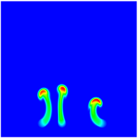 | 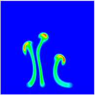 | 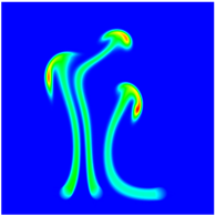 |
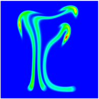 | 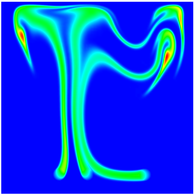 |  | 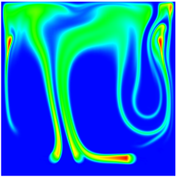 |
The visualizations shown here were generated using a version of the example which did not enforce the constraints after transferring the mesh.
As can be seen, we have three heat sources that heat fluid and therefore produce a buoyancy effect that lets hots pockets of fluid rise up and swirl around. By a chimney effect, the three streams are pressed together by fluid that comes from the outside and wants to join the updraft party. Note that because the fluid is initially at rest, those parts of the fluid that were initially over the sources receive a longer heating time than that fluid that is later dragged over the source by the fully developed flow field. It is therefore hotter, a fact that can be seen in the red tips of the three plumes. Note also the relatively fine features of the flow field, a result of the sophisticated transport stabilization of the temperature equation we have chosen.
In addition to the pictures above, the following ones show the adaptive mesh and the flow field at the same time steps:
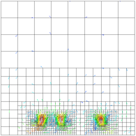 | 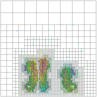 | 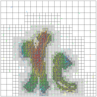 | 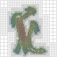 |
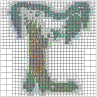 | 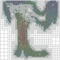 | 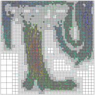 | 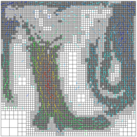 |
The same thing can of course be done in 3d by changing the template parameter to the BoussinesqFlowProblem object in main() from 2 to 3, so that the output now looks like follows:
Number of active cells: 64 (on 3 levels)
Number of degrees of freedom: 3041 (2187+125+729)

Timestep 0:  t=0
   Assembling...
   Rebuilding Stokes preconditioner...
   Solving...
   0 GMRES iterations for Stokes subsystem.
   Time step: 2.45098
   9 CG iterations for temperature.
   Temperature range: -0.675683 4.94725

Number of active cells: 288 (on 4 levels)
Number of degrees of freedom: 12379 (8943+455+2981)

Timestep 0:  t=0
   Assembling...
   Rebuilding Stokes preconditioner...
   Solving...
   0 GMRES iterations for Stokes subsystem.
   Time step: 1.22549
   9 CG iterations for temperature.
   Temperature range: -0.527701 2.25764

Number of active cells: 1296 (on 5 levels)
Number of degrees of freedom: 51497 (37305+1757+12435)

Timestep 0:  t=0
   Assembling...
   Rebuilding Stokes preconditioner...
   Solving...
   0 GMRES iterations for Stokes subsystem.
   Time step: 0.612745
   10 CG iterations for temperature.
   Temperature range: -0.496942 0.847395

Number of active cells: 5048 (on 6 levels)
Number of degrees of freedom: 192425 (139569+6333+46523)

Timestep 0:  t=0
   Assembling...
   Rebuilding Stokes preconditioner...
   Solving...
   0 GMRES iterations for Stokes subsystem.
   Time step: 0.306373
   10 CG iterations for temperature.
   Temperature range: -0.267683 0.497739

Timestep 1:  t=0.306373
   Assembling...
   Solving...
   27 GMRES iterations for Stokes subsystem.
   Time step: 0.306373
   10 CG iterations for temperature.
   Temperature range: -0.461787 0.958679

...
Visualizing the temperature isocontours at time steps 0, 50, 100, 150, 200, 300, 400, 500, 600, 700, and 800 yields the following plots:
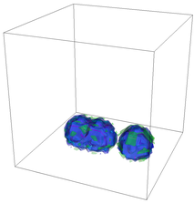 | 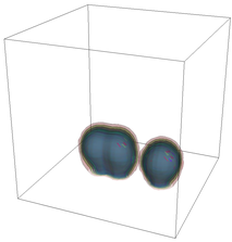 | 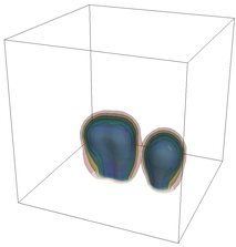 | 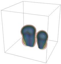 |
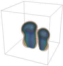 | 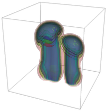 | 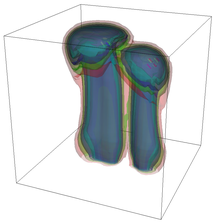 | 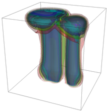 |
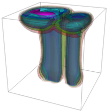 | 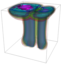 | 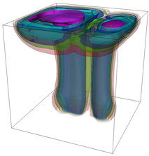 |
That the first picture looks like three hedgehogs stems from the fact that our scheme essentially projects the source times the first time step size onto the mesh to obtain the temperature field in the first time step. Since the source function is discontinuous, we need to expect over- and undershoots from this project. This is in fact what happens (it's easier to check this in 2d) and leads to the crumpled appearance of the isosurfaces. The visualizations shown here were generated using a version of the example which did not enforce the constraints after transferring the mesh.
The program as is has three parameters that we don't have much of a theoretical handle on how to choose in an optimal way. These are:
\begin{eqnarray*} \nu_\alpha(T)|_K = \beta \|\mathbf{u}\|_{L^\infty(K)} \min\left\{ h_K, h_K^\alpha \frac{\|R_\alpha(T)\|_{L^\infty(K)}}{c(\mathbf{u},T)} \right\}, \end{eqnarray*}
with c(\mathbf{u},T) = c_R\ \|\mathbf{u}\|_{L^\infty(\Omega)} \ \mathrm{var}(T) \ |\mathrm{diam}(\Omega)|^{\alpha-2}. Here, the choice of the dimensionless numbers \beta,c_R is of interest.In all of these cases, we will have to expect that the correct choice of each value depends on that of the others, and most likely also on the space dimension and polynomial degree of the finite element used for the temperature. Below we'll discuss a few numerical experiments to choose constants c_k and \beta.
Below, we will not discuss the choice of c_R. In the program, we set it to c_R=2^{\frac{4-2\alpha}{d}}. The reason for this value is a bit complicated and has more to do with the history of the program than reasoning: while the correct formula for the global scaling parameter c(\mathbf{u},T) is shown above, the program (including the version shipped with deal.II 6.2) initially had a bug in that we computed c(\mathbf{u},T) = \|\mathbf{u}\|_{L^\infty(\Omega)} \ \mathrm{var}(T) \ \frac{1}{|\mathrm{diam}(\Omega)|^{\alpha-2}} instead, where we had set the scaling parameter to one. Since we only computed on the unit square/cube where \mathrm{diam}(\Omega)=2^{1/d}, this was entirely equivalent to using the correct formula with c_R=\left(2^{1/d}\right)^{4-2\alpha}=2^{\frac{4-2\alpha}{d}}. Since this value for c_R appears to work just fine for the current program, we corrected the formula in the program and set c_R to a value that reproduces exactly the results we had before. We will, however, revisit this issue again in step-32.
Now, however, back to the discussion of what values of c_k and \beta to choose:
These two constants are definitely linked in some way. The reason is easy to see: In the case of a pure advection problem, \frac{\partial T}{\partial t} + \mathbf{u}\cdot\nabla T = \gamma, any explicit scheme has to satisfy a CFL condition of the form k\le \min_K \frac{c_k^a h_K}{\|\mathbf{u}\|_{L^\infty(K)}}. On the other hand, for a pure diffusion problem, \frac{\partial T}{\partial t} + \nu \Delta T = \gamma, explicit schemes need to satisfy a condition k\le \min_K \frac{c_k^d h_K^2}{\nu}. So given the form of \nu above, an advection diffusion problem like the one we have to solve here will result in a condition of the form k\le \min_K \min \left\{ \frac{c_k^a h_K}{\|\mathbf{u}\|_{L^\infty(K)}}, \frac{c_k^d h_K^2}{\beta \|\mathbf{u}\|_{L^\infty(K)} h_K}\right\} = \min_K \left( \min \left\{ c_k^a, \frac{c_k^d}{\beta}\right\} \frac{h_K}{\|\mathbf{u}\|_{L^\infty(K)}} \right) . It follows that we have to face the fact that we might want to choose \beta larger to improve the stability of the numerical scheme (by increasing the amount of artificial diffusion), but we have to pay a price in the form of smaller, and consequently more time steps. In practice, one would therefore like to choose \beta as small as possible to keep the transport problem sufficiently stabilized while at the same time trying to choose the time step as large as possible to reduce the overall amount of work.
The find the right balance, the only way is to do a few computational experiments. Here's what we did: We modified the program slightly to allow less mesh refinement (so we don't always have to wait that long) and to choose \nu(T)|_K = \beta \|\mathbf{u}\|_{L^\infty(K)} h_K to eliminate the effect of the constant c_R (we know that solutions are stable by using this version of \nu(T) as an artificial viscosity, but that we can improve things – i.e. make the solution sharper – by using the more complicated formula for this artificial viscosity). We then run the program for different values c_k,\beta and observe maximal and minimal temperatures in the domain. What we expect to see is this: If we choose the time step too big (i.e. choose a c_k bigger than theoretically allowed) then we will get exponential growth of the temperature. If we choose \beta too small, then the transport stabilization becomes insufficient and the solution will show significant oscillations but not exponential growth.
Here is what we get for \beta=0.01, \beta=0.1, and \beta=0.5, different choices of c_k, and bilinear elements (temperature_degree=1) in 2d:
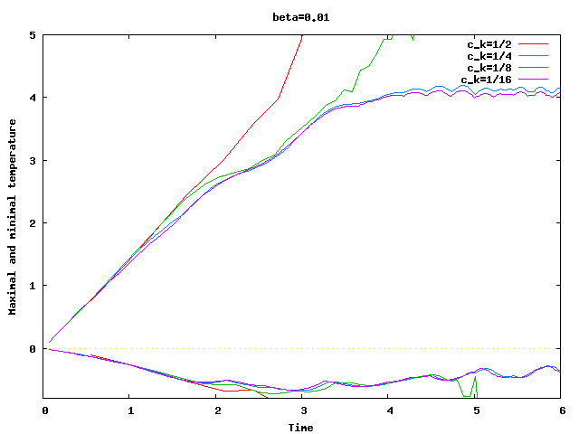 | 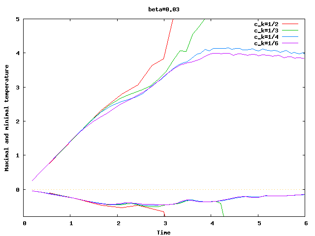 |
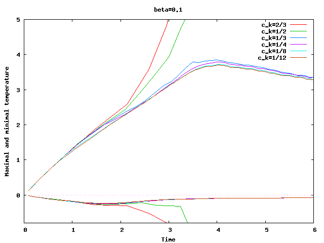 | 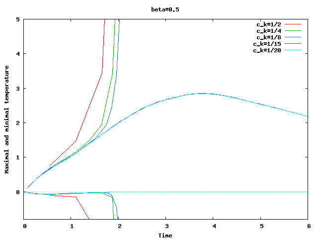 |
The way to interpret these graphs goes like this: for \beta=0.01 and c_k=\frac 12,\frac 14, we see exponential growth or at least large variations, but if we choose k=\frac 18\frac{h_K}{\|\mathbf{u}\|_{L^\infty(K)}} or smaller, then the scheme is stable though a bit wobbly. For more artificial diffusion, we can choose k=\frac 14\frac{h_K}{\|\mathbf{u}\|_{L^\infty(K)}} or smaller for \beta=0.03, k=\frac 13\frac{h_K}{\|\mathbf{u}\|_{L^\infty(K)}} or smaller for \beta=0.1, and again need k=\frac 1{15}\frac{h_K}{\|\mathbf{u}\|_{L^\infty(K)}} for \beta=0.5 (this time because much diffusion requires a small time step).
So how to choose? If we were simply interested in a large time step, then we would go with \beta=0.1 and k=\frac 13\frac{h_K}{\|\mathbf{u}\|_{L^\infty(K)}}. On the other hand, we're also interested in accuracy and here it may be of interest to actually investigate what these curves show. To this end note that we start with a zero temperature and that our sources are positive — so we would intuitively expect that the temperature can never drop below zero. But it does, a consequence of Gibb's phenomenon when using continuous elements to approximate a discontinuous solution. We can therefore see that choosing \beta too small is bad: too little artificial diffusion leads to over- and undershoots that aren't diffused away. On the other hand, for large \beta, the minimum temperature drops below zero at the beginning but then quickly diffuses back to zero.
On the other hand, let's also look at the maximum temperature. Watching the movie of the solution, we see that initially the fluid is at rest. The source keeps heating the same volume of fluid whose temperature increases linearly at the beginning until its buoyancy is able to move it upwards. The hottest part of the fluid is therefore transported away from the solution and fluid taking its place is heated for only a short time before being moved out of the source region, therefore remaining cooler than the initial bubble. If \kappa=0 (in the program it is nonzero but very small) then the hottest part of the fluid should be advected along with the flow with its temperature constant. That's what we can see in the graphs with the smallest \beta: Once the maximum temperature is reached, it hardly changes any more. On the other hand, the larger the artificial diffusion, the more the hot spot is diffused. Note that for this criterion, the time step size does not play a significant role.
So to sum up, likely the best choice would appear to be \beta=0.03 and k=\frac 14\frac{h_K}{\|\mathbf{u}\|_{L^\infty(K)}}. The curve is a bit wobbly, but overall pictures looks pretty reasonable with the exception of some over and undershoots close to the start time due to Gibb's phenomenon.
One can repeat the same sequence of experiments for higher order elements as well. Here are the graphs for bi-quadratic shape functions (temperature_degree=2) for the temperature, while we retain the Q_2/Q_1 stable Taylor-Hood element for the Stokes system:
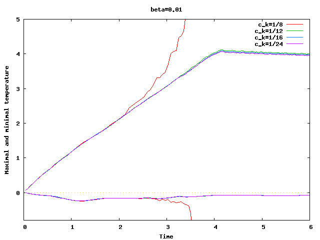 | 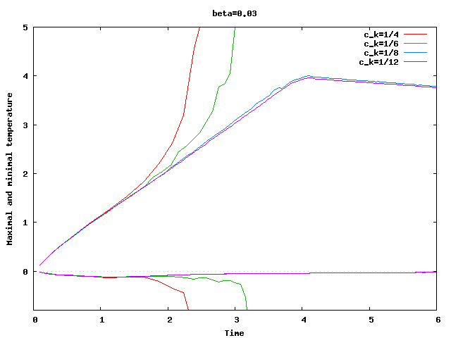 |
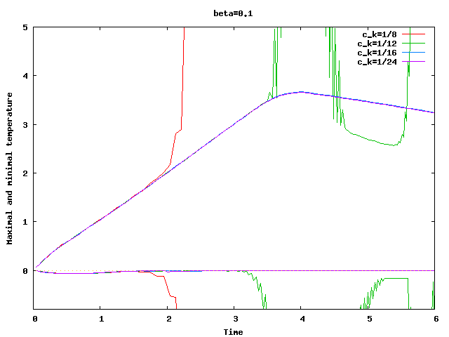 |
Again, small values of \beta lead to less diffusion but we have to choose the time step very small to keep things under control. Too large values of \beta make for more diffusion, but again require small time steps. The best value would appear to be \beta=0.03, as for the Q_1 element, and then we have to choose k=\frac 18\frac{h_K}{\|\mathbf{u}\|_{L^\infty(K)}} — exactly half the size for the Q_1 element, a fact that may not be surprising if we state the CFL condition as the requirement that the time step be small enough so that the distance transport advects in each time step is no longer than one grid point away (which for Q_1 elements is h_K, but for Q_2 elements is h_K/2). It turns out that \beta needs to be slightly larger for obtaining stable results also late in the simulation at times larger than 60, so we actually choose it as \beta = 0.034 in the code.
One can repeat these experiments in 3d and find the optimal time step for each value of \beta and find the best value of \beta. What one finds is that for the same \beta already used in 2d, the time steps needs to be a bit smaller, by around a factor of 1.2 or so. This is easily explained: the time step restriction is k=\min_K \frac{ch_K}{\|\mathbf{u}\|_{L^\infty(K)}} where h_K is the diameter of the cell. However, what is really needed is the distance between mesh points, which is \frac{h_K}{\sqrt{d}}. So a more appropriate form would be k=\min_K \frac{ch_K}{\|\mathbf{u}\|_{L^\infty(K)}\sqrt{d}}.
The second find is that one needs to choose \beta slightly bigger (about \beta=0.05 or so). This then again reduces the time step we can take.
Concluding, from the simple computations above, \beta=0.034 appears to be a good choice for the stabilization parameter in 2d, and \beta=0.05 in 3d. In a dimension independent way, we can model this as \beta=0.017d. If one does longer computations (several thousand time steps) on finer meshes, one realizes that the time step size is not quite small enough and that for stability one will have to reduce the above values a bit more (by about a factor of \frac 78).
As a consequence, a formula that reconciles 2d, 3d, and variable polynomial degree and takes all factors in account reads as follows:
\begin{eqnarray*} k = \frac 1{2 \cdot 1.7} \frac 1{\sqrt{d}} \frac 2d \frac 1{q_T} \frac{h_K}{\|\mathbf{u}\|_{L^\infty(K)}} = \frac 1{1.7 d\sqrt{d}} \frac 1{q_T} \frac{h_K}{\|\mathbf{u}\|_{L^\infty(K)}}. \end{eqnarray*}
In the first form (in the center of the equation), \frac 1{2 \cdot 1.7} is a universal constant, \frac 1{\sqrt{d}} is the factor that accounts for the difference between cell diameter and grid point separation, \frac 2d accounts for the increase in \beta with space dimension, \frac 1{q_T} accounts for the distance between grid points for higher order elements, and \frac{h_K}{\|\mathbf{u}\|_{L^\infty(K)}} for the local speed of transport relative to the cell size. This is the formula that we use in the program.
As for the question of whether to use Q_1 or Q_2 elements for the temperature, the following considerations may be useful: First, solving the temperature equation is hardly a factor in the overall scheme since almost the entire compute time goes into solving the Stokes system in each time step. Higher order elements for the temperature equation are therefore not a significant drawback. On the other hand, if one compares the size of the over- and undershoots the solution produces due to the discontinuous source description, one notices that for the choice of \beta and k as above, the Q_1 solution dips down to around -0.47, whereas the Q_2 solution only goes to -0.13 (remember that the exact solution should never become negative at all. This means that the Q_2 solution is significantly more accurate; the program therefore uses these higher order elements, despite the penalty we pay in terms of smaller time steps.
There are various ways to extend the current program. Of particular interest is, of course, to make it faster and/or increase the resolution of the program, in particular in 3d. This is the topic of the step-32 tutorial program which will implement strategies to solve this problem in parallel on a cluster. It is also the basis of the much larger open source code ASPECT (see https://aspect.geodynamics.org/ ) that can solve realistic problems and that constitutes the further development of step-32.
Another direction would be to make the fluid flow more realistic. The program was initially written to simulate various cases simulating the convection of material in the earth's mantle, i.e. the zone between the outer earth core and the solid earth crust: there, material is heated from below and cooled from above, leading to thermal convection. The physics of this fluid are much more complicated than shown in this program, however: The viscosity of mantle material is strongly dependent on the temperature, i.e. \eta=\eta(T), with the dependency frequently modeled as a viscosity that is reduced exponentially with rising temperature. Secondly, much of the dynamics of the mantle is determined by chemical reactions, primarily phase changes of the various crystals that make up the mantle; the buoyancy term on the right hand side of the Stokes equations then depends not only on the temperature, but also on the chemical composition at a given location which is advected by the flow field but also changes as a function of pressure and temperature. We will investigate some of these effects in later tutorial programs as well.