 |
Reference documentation for deal.II version 9.1.1
|
 |
Reference documentation for deal.II version 9.1.1
|
This tutorial depends on step-6, step-21.
| Table of contents | |
|---|---|
This program was contributed by Martin Kronbichler and Wolfgang Bangerth.
This material is based upon work partly supported by the National Science Foundation under Award No. EAR-0426271 and The California Institute of Technology. Any opinions, findings, and conclusions or recommendations expressed in this publication are those of the author and do not necessarily reflect the views of the National Science Foundation or of The California Institute of Technology.
This program deals with the Stokes system of equations which reads as follows in non-dimensionalized form:
\begin{eqnarray*} -2\; \textrm{div}\; \varepsilon(\textbf{u}) + \nabla p &=& \textbf{f}, \\ -\textrm{div}\; \textbf{u} &=& 0, \end{eqnarray*}
where \textbf u denotes the velocity of a fluid, p is its pressure, \textbf f are external forces, and \varepsilon(\textbf{u})= \nabla^s{\textbf{u}}= \frac 12 \left[ (\nabla \textbf{u}) + (\nabla \textbf{u})^T\right] is the rank-2 tensor of symmetrized gradients; a component-wise definition of it is \varepsilon(\textbf{u})_{ij}=\frac 12\left(\frac{\partial u_i}{\partial x_j} + \frac{\partial u_j}{\partial x_i}\right).
The Stokes equations describe the steady-state motion of a slow-moving, viscous fluid such as honey, rocks in the earth mantle, or other cases where inertia does not play a significant role. If a fluid is moving fast enough that inertia forces are significant compared to viscous friction, the Stokes equations are no longer valid; taking into account inertia effects then leads to the nonlinear Navier-Stokes equations. However, in this tutorial program, we will focus on the simpler Stokes system.
Note that when deriving the more general compressible Navier-Stokes equations, the diffusion is modeled as the divergence of the stress tensor
\begin{eqnarray*} \tau = - \mu (2\varepsilon(\textbf{u}) - \frac{2}{3}\nabla \cdot \textbf{u} I), \end{eqnarray*}
where \mu is the viscosity of the fluid. With the assumption of \mu=1 (assume constant viscosity and non-dimensionalize the equation by dividing out \mu) and assuming incompressibility ( \textrm{div}\; \textbf{u}=0), we arrive at the formulation from above:
\begin{eqnarray*} \textrm{div}\; \tau = -2\textrm{div}\;\varepsilon(\textbf{u}). \end{eqnarray*}
A different formulation uses the Laplace operator ( -\triangle \textbf{u}) instead of the symmetrized gradient. A big difference here is that the different components of the velocity do not couple. If you assume additional regularity of the solution \textbf{u} (second partial derivatives exist and are continuous), the formulations are equivalent:
\begin{eqnarray*} \textrm{div}\; \tau = -2\textrm{div}\;\varepsilon(\textbf{u}) = -\triangle \textbf{u} + \nabla \cdot (\nabla\textbf{u})^T = -\triangle \textbf{u}. \end{eqnarray*}
This is because the ith entry of \nabla \cdot (\nabla\textbf{u})^T is given by:
\begin{eqnarray*} [\nabla \cdot (\nabla\textbf{u})^T]_i = \sum_j \frac{\partial}{\partial x_j} [(\nabla\textbf{u})^T]_{i,j} = \sum_j \frac{\partial}{\partial x_j} [(\nabla\textbf{u})]_{j,i} = \sum_j \frac{\partial}{\partial x_j} \frac{\partial}{\partial x_i} \textbf{u}_j = \sum_j \frac{\partial}{\partial x_i} \frac{\partial}{\partial x_j} \textbf{u}_j = \frac{\partial}{\partial x_i} \textrm{div}\; \textbf{u} = 0. \end{eqnarray*}
If you can not assume the above mentioned regularity, or if your viscosity is not a constant, the equivalence no longer holds. Therefore, we decided to stick with the more physically accurate symmetric tensor formulation in this tutorial.
To be well-posed, we will have to add boundary conditions to the equations. What boundary conditions are readily possible here will become clear once we discuss the weak form of the equations.
The equations covered here fall into the class of vector-valued problems. A toplevel overview of this topic can be found in the Handling vector valued problems module.
The weak form of the equations is obtained by writing it in vector form as
\begin{eqnarray*} \begin{pmatrix} {-2\; \textrm{div}\; \varepsilon(\textbf{u}) + \nabla p} \\ {-\textrm{div}\; \textbf{u}} \end{pmatrix} = \begin{pmatrix} {\textbf{f}} \\ 0 \end{pmatrix}, \end{eqnarray*}
forming the dot product from the left with a vector-valued test function \phi = \begin{pmatrix}\textbf{v} \\ q\end{pmatrix} and integrating over the domain \Omega, yielding the following set of equations:
\begin{eqnarray*} (\mathrm v, -2\; \textrm{div}\; \varepsilon(\textbf{u}) + \nabla p)_{\Omega} - (q,\textrm{div}\; \textbf{u})_{\Omega} = (\textbf{v}, \textbf{f})_\Omega, \end{eqnarray*}
which has to hold for all test functions \phi = \begin{pmatrix}\textbf{v} \\ q\end{pmatrix}.
In practice, one wants to impose as little regularity on the pressure variable as possible; consequently, we integrate by parts the second term:
\begin{eqnarray*} (\textbf{v}, -2\; \textrm{div}\; \varepsilon(\textbf{u}))_{\Omega} - (\textrm{div}\; \textbf{v}, p)_{\Omega} + (\textbf{n}\cdot\textbf{v}, p)_{\partial\Omega} - (q,\textrm{div}\; \textbf{u})_{\Omega} = (\textbf{v}, \textbf{f})_\Omega. \end{eqnarray*}
Likewise, we integrate by parts the first term to obtain
\begin{eqnarray*} (\nabla \textbf{v}, 2\; \varepsilon(\textbf{u}))_{\Omega} - (\textbf{n} \otimes \textbf{v}, 2\; \varepsilon(\textbf{u}))_{\partial\Omega} - (\textrm{div}\; \textbf{v}, p)_{\Omega} + (\textbf{n}\cdot\textbf{v}, p)_{\partial\Omega} - (q,\textrm{div}\; \textbf{u})_{\Omega} = (\textbf{v}, \textbf{f})_\Omega, \end{eqnarray*}
where the scalar product between two tensor-valued quantities is here defined as
\begin{eqnarray*} (\nabla \textbf{v}, 2\; \varepsilon(\textbf{u}))_{\Omega} = 2 \int_\Omega \sum_{i,j=1}^d \frac{\partial v_j}{\partial x_i} \varepsilon(\textbf{u})_{ij} \ dx. \end{eqnarray*}
Because the scalar product between a general tensor like \nabla\textbf{v} and a symmetric tensor like \varepsilon(\textbf{u}) equals the scalar product between the symmetrized forms of the two, we can also write the bilinear form above as follows:
\begin{eqnarray*} (\varepsilon(\textbf{v}), 2\; \varepsilon(\textbf{u}))_{\Omega} - (\textbf{n} \otimes \textbf{v}, 2\; \varepsilon(\textbf{u}))_{\partial\Omega} - (\textrm{div}\; \textbf{v}, p)_{\Omega} + (\textbf{n}\cdot\textbf{v}, p)_{\partial\Omega} - (q,\textrm{div}\; \textbf{u})_{\Omega} = (\textbf{v}, \textbf{f})_\Omega, \end{eqnarray*}
We will deal with the boundary terms in the next section, but it is already clear from the domain terms
\begin{eqnarray*} (\varepsilon(\textbf{v}), 2\; \varepsilon(\textbf{u}))_{\Omega} - (\textrm{div}\; \textbf{v}, p)_{\Omega} - (q,\textrm{div}\; \textbf{u})_{\Omega} \end{eqnarray*}
of the bilinear form that the Stokes equations yield a symmetric bilinear form, and consequently a symmetric (if indefinite) system matrix.
The weak form just derived immediately presents us with different possibilities for imposing boundary conditions:
Dirichlet velocity boundary conditions: On a part \Gamma_D\subset\partial\Omega we may impose Dirichlet conditions on the velocity \textbf u:
\begin{eqnarray*} \textbf u = \textbf g_D \qquad\qquad \textrm{on}\ \Gamma_D. \end{eqnarray*}
Because test functions \textbf{v} come from the tangent space of the solution variable, we have that \textbf{v}=0 on \Gamma_D and consequently that
\begin{eqnarray*} -(\textbf{n} \otimes \mathrm v, 2\; \varepsilon(\textbf{u}))_{\Gamma_D} + (\textbf{n}\cdot\textbf{v}, p)_{\Gamma_D} = 0. \end{eqnarray*}
In other words, as usual, strongly imposed boundary values do not appear in the weak form.
It is noteworthy that if we impose Dirichlet boundary values on the entire boundary, then the pressure is only determined up to a constant. An algorithmic realization of that would use similar tools as have been seen in step-11.
Neumann-type or natural boundary conditions: On the rest of the boundary \Gamma_N=\partial\Omega\backslash\Gamma_D, let us re-write the boundary terms as follows:
\begin{eqnarray*} -(\textbf{n} \otimes \mathrm v, 2\; \varepsilon(\textbf{u}))_{\Gamma_N} + (\textbf{n}\cdot\textbf{v}, p)_{\Gamma_N} &=& \sum_{i,j=1}^d -(n_i v_j, 2\; \varepsilon(\textbf{u})_{ij})_{\Gamma_N} + \sum_{i=1}^d (n_i v_i, p)_{\Gamma_N} \\ &=& \sum_{i,j=1}^d -(n_i v_j, 2\; \varepsilon(\textbf{u})_{ij})_{\Gamma_N} + \sum_{i,j=1}^d (n_i v_j, p \delta_{ij})_{\Gamma_N} \\ &=& \sum_{i,j=1}^d (n_i v_j,p \delta_{ij} - 2\; \varepsilon(\textbf{u})_{ij})_{\Gamma_N} \\ &=& (\textbf{n} \otimes \textbf{v}, p \textbf{I} - 2\; \varepsilon(\textbf{u}))_{\Gamma_N}. \\ &=& (\textbf{v}, \textbf{n}\cdot [p \textbf{I} - 2\; \varepsilon(\textbf{u})])_{\Gamma_N}. \end{eqnarray*}
In other words, on the Neumann part of the boundary we can prescribe values for the total stress:
\begin{eqnarray*} \textbf{n}\cdot [p \textbf{I} - 2\; \varepsilon(\textbf{u})] = \textbf g_N \qquad\qquad \textrm{on}\ \Gamma_N. \end{eqnarray*}
If the boundary is subdivided into Dirichlet and Neumann parts \Gamma_D,\Gamma_N, this then leads to the following weak form:
\begin{eqnarray*} (\varepsilon(\textbf{v}), 2\; \varepsilon(\textbf{u}))_{\Omega} - (\textrm{div}\; \textbf{v}, p)_{\Omega} - (q,\textrm{div}\; \textbf{u})_{\Omega} = (\textbf{v}, \textbf{f})_\Omega - (\textbf{v}, \textbf g_N)_{\Gamma_N}. \end{eqnarray*}
Robin-type boundary conditions: Robin boundary conditions are a mixture of Dirichlet and Neumann boundary conditions. They would read
\begin{eqnarray*} \textbf{n}\cdot [p \textbf{I} - 2\; \varepsilon(\textbf{u})] = \textbf S \textbf u \qquad\qquad \textrm{on}\ \Gamma_R, \end{eqnarray*}
with a rank-2 tensor (matrix) \textbf S. The associated weak form is
\begin{eqnarray*} (\varepsilon(\textbf{v}), 2\; \varepsilon(\textbf{u}))_{\Omega} - (\textrm{div}\; \textbf{v}, p)_{\Omega} - (q,\textrm{div}\; \textbf{u})_{\Omega} + (\textbf S \textbf u, \textbf{v})_{\Gamma_R} = (\textbf{v}, \textbf{f})_\Omega. \end{eqnarray*}
Partial boundary conditions: It is possible to combine Dirichlet and Neumann boundary conditions by only enforcing each of them for certain components of the velocity. For example, one way to impose artificial boundary conditions is to require that the flow is perpendicular to the boundary, i.e. the tangential component \textbf u_{\textbf t}=(\textbf 1-\textbf n\otimes\textbf n)\textbf u be zero, thereby constraining dim-1 components of the velocity. The remaining component can be constrained by requiring that the normal component of the normal stress be zero, yielding the following set of boundary conditions:
\begin{eqnarray*} \textbf u_{\textbf t} &=& 0, \\ \textbf n \cdot \left(\textbf{n}\cdot [p \textbf{I} - 2\; \varepsilon(\textbf{u})] \right) &=& 0. \end{eqnarray*}
An alternative to this is when one wants the flow to be parallel rather than perpendicular to the boundary (in deal.II, the VectorTools::compute_no_normal_flux_constraints function can do this for you). This is frequently the case for problems with a free boundary (e.g. at the surface of a river or lake if vertical forces of the flow are not large enough to actually deform the surface), or if no significant friction is exerted by the boundary on the fluid (e.g. at the interface between earth mantle and earth core where two fluids meet that are stratified by different densities but that both have small enough viscosities to not introduce much tangential stress on each other). In formulas, this means that
\begin{eqnarray*} \textbf{n}\cdot\textbf u &=& 0, \\ (\textbf 1-\textbf n\otimes\textbf n) \left(\textbf{n}\cdot [p \textbf{I} - 2\; \varepsilon(\textbf{u})] \right) &=& 0, \end{eqnarray*}
the first condition (which needs to be imposed strongly) fixing a single component of the velocity, with the second (which would be enforced in the weak form) fixing the remaining two components.
Despite this wealth of possibilities, we will only use Dirichlet and (homogeneous) Neumann boundary conditions in this tutorial program.
As developed above, the weak form of the equations with Dirichlet and Neumann boundary conditions on \Gamma_D and \Gamma_N reads like this: find \textbf u\in \textbf V_g = \{\varphi \in H^1(\Omega)^d: \varphi_{\Gamma_D}=\textbf g_D\}, p\in Q=L^2(\Omega) so that
\begin{eqnarray*} (\varepsilon(\textbf{v}), 2\; \varepsilon(\textbf{u}))_{\Omega} - (\textrm{div}\; \textbf{v}, p)_{\Omega} - (q,\textrm{div}\; \textbf{u})_{\Omega} = (\textbf{v}, \textbf{f})_\Omega - (\textbf{v}, \textbf g_N)_{\Gamma_N} \end{eqnarray*}
for all test functions \textbf{v}\in \textbf V_0 = \{\varphi \in H^1(\Omega)^d: \varphi_{\Gamma_D}=0\},q\in Q.
These equations represent a symmetric saddle point problem. It is well known that then a solution only exists if the function spaces in which we search for a solution have to satisfy certain conditions, typically referred to as the Babuska-Brezzi or Ladyzhenskaya-Babuska-Brezzi (LBB) conditions. The continuous function spaces above satisfy them. However, when we discretize the equations by replacing the continuous variables and test functions by finite element functions in finite dimensional spaces \textbf V_{g,h}\subset \textbf V_g, Q_h\subset Q, we have to make sure that \textbf V_h,Q_h also satisfy the LBB conditions. This is similar to what we had to do in step-20.
For the Stokes equations, there are a number of possible choices to ensure that the finite element spaces are compatible with the LBB condition. A simple and accurate choice that we will use here is \textbf u_h\in Q_{p+1}^d, p_h\in Q_p, i.e. use elements one order higher for the velocities than for the pressures.
This then leads to the following discrete problem: find \textbf u_h,p_h so that
\begin{eqnarray*} (\varepsilon(\textbf{v}_h), 2\; \varepsilon(\textbf u_h))_{\Omega} - (\textrm{div}\; \textbf{v}_h, p_h)_{\Omega} - (q_h,\textrm{div}\; \textbf{u}_h)_{\Omega} = (\textbf{v}_h, \textbf{f})_\Omega - (\textbf{v}_h, \textbf g_N)_{\Gamma_N} \end{eqnarray*}
for all test functions \textbf{v}_h, q_h. Assembling the linear system associated with this problem follows the same lines used in step-20, step-21, and explained in detail in the Handling vector valued problems module.
The weak form of the discrete equations naturally leads to the following linear system for the nodal values of the velocity and pressure fields:
\begin{eqnarray*} \left(\begin{array}{cc} A & B^T \\ B & 0 \end{array}\right) \left(\begin{array}{c} U \\ P \end{array}\right) = \left(\begin{array}{c} F \\ G \end{array}\right), \end{eqnarray*}
Like in step-20 and step-21, we will solve this system of equations by forming the Schur complement, i.e. we will first find the solution P of
\begin{eqnarray*} BA^{-1}B^T P &=& BA^{-1} F - G, \\ \end{eqnarray*}
and then
\begin{eqnarray*} AU &=& F - B^TP. \end{eqnarray*}
The way we do this is pretty much exactly like we did in these previous tutorial programs, i.e. we use the same classes SchurComplement and InverseMatrix again. There are two significant differences, however:
First, in the mixed Laplace equation we had to deal with the question of how to precondition the Schur complement B^TM^{-1}B, which was spectrally equivalent to the Laplace operator on the pressure space (because B represents the gradient operator, B^T its adjoint -\textrm{div}, and M the identity (up to the material parameter K^{-1}), so B^TM^{-1}B is something like -\textrm{div} \mathbf 1 \nabla = -\Delta). Consequently, the matrix is badly conditioned for small mesh sizes and we had to come up with an elaborate preconditioning scheme for the Schur complement.
In other words, preconditioning the inner solver for M was simple whereas preconditioning the outer solver for B^TM^{-1}B was complicated.
Here, the situation is pretty much exactly the opposite. The difference stems from the fact that the matrix at the heart of the Schur complement does not stem from the identity operator but from a variant of the Laplace operator, -\textrm{div} \nabla^s (where \nabla^s is the symmetric gradient) acting on a vector field. In the investigation of this issue we largely follow the paper D. Silvester and A. Wathen: "Fast iterative solution of stabilised Stokes systems part II. Using general block preconditioners." (SIAM J. Numer. Anal., 31 (1994), pp. 1352-1367), which is available online here. Principally, the difference in the matrix at the heart of the Schur complement has two consequences:
First, it makes the outer preconditioner simple: the Schur complement corresponds to the operator -\textrm{div} (-\textrm{div} \nabla^s)^{-1} \nabla on the pressure space; forgetting about the fact that we deal with symmetric gradients instead of the regular one, the Schur complement is something like -\textrm{div} (-\textrm{div} \nabla)^{-1} \nabla = -\textrm{div} (-\Delta)^{-1} \nabla, which, even if not mathematically entirely concise, is spectrally equivalent to the identity operator (a heuristic argument would be to commute the operators into -\textrm{div}(-\Delta)^{-1} \nabla = -\textrm{div}\nabla(-\Delta)^{-1} = -\Delta(-\Delta)^{-1} = \mathbf 1). It turns out that it isn't easy to solve this Schur complement in a straightforward way with the CG method: using no preconditioner, the condition number of the Schur complement matrix depends on the size ratios of the largest to the smallest cells, and one still needs on the order of 50-100 CG iterations. However, there is a simple cure: precondition with the mass matrix on the pressure space and we get down to a number between 5-15 CG iterations, pretty much independently of the structure of the mesh (take a look at the results section of this program to see that indeed the number of CG iterations does not change as we refine the mesh).
So all we need in addition to what we already have is the mass matrix on the pressure variables and we will store it in a separate object.
While the outer preconditioner has become simpler compared to the mixed Laplace case discussed in step-20, the issue of the inner solver has become more complicated. In the mixed Laplace discretization, the Schur complement has the form B^TM^{-1}B. Thus, every time we multiplied with the Schur complement, we had to solve a linear system M_uz=y; this isn't too complicated there, however, since the mass matrix M_u on the pressure space is well-conditioned.
On the other hand, for the Stokes equation we consider here, the Schur complement is BA^{-1}B^T where the matrix A is related to the Laplace operator (it is, in fact, the matrix corresponding to the bilinear form (\nabla^s \varphi_i, \nabla^s\varphi_j)). Thus, solving with A is a lot more complicated: the matrix is badly conditioned and we know that we need many iterations unless we have a very good preconditioner. What is worse, we have to solve with A every time we multiply with the Schur complement, which is 5-15 times using the preconditioner described above.
Because we have to solve with A several times, it pays off to spend a bit more time once to create a good preconditioner for this matrix. So here's what we're going to do: if in 2d, we use the ultimate preconditioner, namely a direct sparse LU decomposition of the matrix. This is implemented using the SparseDirectUMFPACK class that uses the UMFPACK direct solver to compute the decomposition. To use it, you will have to build deal.II with UMFPACK support (which is the default); see the ReadMe file for instructions. With this, the inner solver converges in one iteration.
In 2d, we can do this sort of thing because even reasonably large problems rarely have more than a few 100,000 unknowns with relatively few nonzero entries per row. Furthermore, the bandwidth of matrices in 2d is {\cal O}(\sqrt{N}) and therefore moderate. For such matrices, sparse factors can be computed in a matter of a few seconds. (As a point of reference, computing the sparse factors of a matrix of size N and bandwidth B takes {\cal O}(NB^2) operations. In 2d, this is {\cal O}(N^2); though this is a higher complexity than, for example, assembling the linear system which takes {\cal O}(N), the constant for computing the decomposition is so small that it doesn't become the dominating factor in the entire program until we get to very large numbers of unknowns in the high 100,000s or more.)
The situation changes in 3d, because there we quickly have many more unknowns and the bandwidth of matrices (which determines the number of nonzero entries in sparse LU factors) is {\cal O}(N^{2/3}), and there are many more entries per row as well. This makes using a sparse direct solver such as UMFPACK inefficient: only for problem sizes of a few 10,000 to maybe 100,000 unknowns can a sparse decomposition be computed using reasonable time and memory resources.
What we do in that case is to use an incomplete LU decomposition (ILU) as a preconditioner, rather than actually computing complete LU factors. As it so happens, deal.II has a class that does this: SparseILU. Computing the ILU takes a time that only depends on the number of nonzero entries in the sparse matrix (or that we are willing to fill in the LU factors, if these should be more than the ones in the matrix), but is independent of the bandwidth of the matrix. It is therefore an operation that can efficiently also be computed in 3d. On the other hand, an incomplete LU decomposition, by definition, does not represent an exact inverse of the matrix A. Consequently, preconditioning with the ILU will still require more than one iteration, unlike preconditioning with the sparse direct solver. The inner solver will therefore take more time when multiplying with the Schur complement: an unavoidable trade-off.
In the program below, we will make use of the fact that the SparseILU and SparseDirectUMFPACK classes have a very similar interface and can be used interchangeably. All that we need is a switch class that, depending on the dimension, provides a type that is either of the two classes mentioned above. This is how we do that:
From here on, we can refer to the type typename InnerPreconditioner<dim>::type and automatically get the correct preconditioner class. Because of the similarity of the interfaces of the two classes, we will be able to use them interchangeably using the same syntax in all places.
The domain, right hand side and boundary conditions we implement below relate to a problem in geophysics: there, one wants to compute the flow field of magma in the earth's interior under a mid-ocean rift. Rifts are places where two continental plates are very slowly drifting apart (a few centimeters per year at most), leaving a crack in the earth crust that is filled with magma from below. Without trying to be entirely realistic, we model this situation by solving the following set of equations and boundary conditions on the domain \Omega=[-2,2]\times[0,1]\times[-1,0]:
\begin{eqnarray*} -2\; \textrm{div}\; \varepsilon(\textbf{u}) + \nabla p &=& 0, \\ -\textrm{div}\; \textbf{u} &=& 0, \\ \mathbf u &=& \left(\begin{array}{c} -1 \\ 0 \\0 \end{array}\right) \qquad\qquad \textrm{at}\ z=0, x<0, \\ \mathbf u &=& \left(\begin{array}{c} +1 \\ 0 \\0 \end{array}\right) \qquad\qquad \textrm{at}\ z=0, x>0, \\ \mathbf u &=& \left(\begin{array}{c} 0 \\ 0 \\0 \end{array}\right) \qquad\qquad \textrm{at}\ z=0, x=0, \end{eqnarray*}
and using natural boundary conditions \textbf{n}\cdot [p \textbf{I} - 2 \varepsilon(\textbf{u})] = 0 everywhere else. In other words, at the left part of the top surface we prescribe that the fluid moves with the continental plate to the left at speed -1, that it moves to the right on the right part of the top surface, and impose natural flow conditions everywhere else. If we are in 2d, the description is essentially the same, with the exception that we omit the second component of all vectors stated above.
As will become apparent in the results section, the flow field will pull material from below and move it to the left and right ends of the domain, as expected. The discontinuity of velocity boundary conditions will produce a singularity in the pressure at the center of the top surface that sucks material all the way to the top surface to fill the gap left by the outward motion of material at this location.
In all the previous tutorial programs, we used the AffineConstraints object merely for handling hanging node constraints (with exception of step-11). However, the class can also be used to implement Dirichlet boundary conditions, as we will show in this program, by fixing some node values x_i = b_i. Note that these are inhomogeneous constraints, and we have to pay some special attention to that. The way we are going to implement this is to first read in the boundary values into the AffineConstraints object by using the call
very similar to how we were making the list of boundary nodes before (note that we set Dirichlet conditions only on boundaries with boundary flag 1). The actual application of the boundary values is then handled by the AffineConstraints object directly, without any additional interference.
We could then proceed as before, namely by filling the matrix, and then calling a condense function on the constraints object of the form
Note that we call this on the system matrix and system right hand side simultaneously, since resolving inhomogeneous constraints requires knowledge about both the matrix entries and the right hand side. For efficiency reasons, though, we choose another strategy: all the constraints collected in the AffineConstraints object can be resolved on the fly while writing local data into the global matrix, by using the call
This technique is further discussed in the step-27 tutorial program. All we need to know here is that this functions does three things at once: it writes the local data into the global matrix and right hand side, it distributes the hanging node constraints and additionally implements (inhomogeneous) Dirichlet boundary conditions. That's nice, isn't it?
We can conclude that the AffineConstraints class provides an alternative to using MatrixTools::apply_boundary_values for implementing Dirichlet boundary conditions.
Frequently, a sparse matrix contains a substantial amount of elements that actually are zero when we are about to start a linear solve. Such elements are introduced when we eliminate constraints or implement Dirichlet conditions, where we usually delete all entries in constrained rows and columns, i.e., we set them to zero. The fraction of elements that are present in the sparsity pattern, but do not really contain any information, can be up to one fourth of the total number of elements in the matrix for the 3D application considered in this tutorial program. Remember that matrix-vector products or preconditioners operate on all the elements of a sparse matrix (even those that are zero), which is an inefficiency we will avoid here.
An advantage of directly resolving constrained degrees of freedom is that we can avoid having most of the entries that are going to be zero in our sparse matrix — we do not need constrained entries during matrix construction (as opposed to the traditional algorithms, which first fill the matrix, and only resolve constraints afterwards). This will save both memory and time when forming matrix-vector products. The way we are going to do that is to pass the information about constraints to the function that generates the sparsity pattern, and then set a false argument specifying that we do not intend to use constrained entries:
This functions obviates, by the way, also the call to the condense() function on the sparsity pattern.
The program developed below has seen a lot of TLC. We have run it over and over under profiling tools (mainly valgrind's cachegrind and callgrind tools, as well as the KDE KCachegrind program for visualization) to see where the bottlenecks are. This has paid off: through this effort, the program has become about four times as fast when considering the runtime of the refinement cycles zero through three, reducing the overall number of CPU instructions executed from 869,574,060,348 to 199,853,005,625. For higher refinement levels, the gain is probably even larger since some algorithms that are not {\cal O}(N) have been eliminated.
Essentially, there are currently two algorithms in the program that do not scale linearly with the number of degrees of freedom: renumbering of degrees of freedom (which is {\cal O}(N \log N), and the linear solver (which is {\cal O}(N^{4/3})). As for the first, while reordering degrees of freedom may not scale linearly, it is an indispensable part of the overall algorithm as it greatly improves the quality of the sparse ILU, easily making up for the time spent on computing the renumbering; graphs and timings to demonstrate this are shown in the documentation of the DoFRenumbering namespace, also underlining the choice of the Cuthill-McKee reordering algorithm chosen below.
As for the linear solver: as mentioned above, our implementation here uses a Schur complement formulation. This is not necessarily the very best choice but demonstrates various important techniques available in deal.II. The question of which solver is best is again discussed in the section on improved solvers in the results part of this program, along with code showing alternative solvers and a comparison of their results.
Apart from this, many other algorithms have been tested and improved during the creation of this program. For example, in building the sparsity pattern, we originally used a (now no longer existing) BlockCompressedSparsityPattern object that added one element at a time; however, its data structures were poorly adapted for the large numbers of nonzero entries per row created by our discretization in 3d, leading to a quadratic behavior. Replacing the internal algorithms in deal.II to set many elements at a time, and using a BlockCompressedSimpleSparsityPattern (which has, as of early 2015, been in turn replaced by BlockDynamicSparsityPattern) as a better adapted data structure, removed this bottleneck at the price of a slightly higher memory consumption. Likewise, the implementation of the decomposition step in the SparseILU class was very inefficient and has been replaced by one that is about 10 times faster. Even the vmult function of the SparseILU has been improved to save about twenty percent of time. Small improvements were applied here and there. Moreover, the AffineConstraints object has been used to eliminate a lot of entries in the sparse matrix that are eventually going to be zero, see the section on using advanced features of the AffineConstraints class.
A profile of how many CPU instructions are spent at the various different places in the program during refinement cycles zero through three in 3d is shown here:
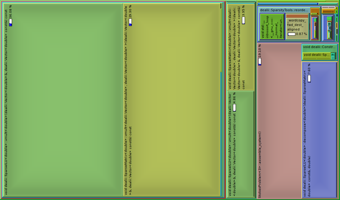
As can be seen, at this refinement level approximately three quarters of the instruction count is spent on the actual solver (the SparseILU::vmult calls on the left, the SparseMatrix::vmult call in the middle for the Schur complement solve, and another box representing the multiplications with SparseILU and SparseMatrix in the solve for U). About one fifth of the instruction count is spent on matrix assembly and sparse ILU computation (box in the lower right corner) and the rest on other things. Since floating point operations such as in the SparseILU::vmult calls typically take much longer than many of the logical operations and table lookups in matrix assembly, the fraction of the run time taken up by matrix assembly is actually significantly less than the fraction of instructions, as will become apparent in the comparison we make in the results section.
For higher refinement levels, the boxes representing the solver as well as the blue box at the top right stemming from reordering algorithm are going to grow at the expense of the other parts of the program, since they don't scale linearly. The fact that at this moderate refinement level (3168 cells and 93176 degrees of freedom) the linear solver already makes up about three quarters of the instructions is a good sign that most of the algorithms used in this program are well-tuned and that major improvements in speeding up the program are most likely not to come from hand-optimizing individual aspects but by changing solver algorithms. We will address this point in the discussion of results below as well.
As a final point, and as a point of reference, the following picture also shows how the profile looked at an early stage of optimizing this program:
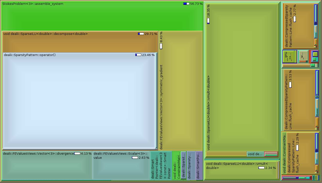
As mentioned above, the runtime of this version was about four times as long as for the first profile, with the SparseILU decomposition taking up about 30% of the instruction count, and operations an early, inefficient version of DynamicSparsityPattern about 10%. Both these bottlenecks have since been completely removed.
As usual, we start by including some well-known files:
Then we need to include the header file for the sparse direct solver UMFPACK:
This includes the library for the incomplete LU factorization that will be used as a preconditioner in 3D:
This is C++:
As in all programs, the namespace dealii is included:
As explained in the introduction, we are going to use different preconditioners for two and three space dimensions, respectively. We distinguish between them by the use of the spatial dimension as a template parameter. See step-4 for details on templates. We are not going to create any preconditioner object here, all we do is to create class that holds a local alias determining the preconditioner class so we can write our program in a dimension-independent way.
In 2D, we are going to use a sparse direct solver as preconditioner:
And the ILU preconditioning in 3D, called by SparseILU:
StokesProblem class templateThis is an adaptation of step-20, so the main class and the data types are nearly the same as used there. The only difference is that we have an additional member preconditioner_matrix, that is used for preconditioning the Schur complement, and a corresponding sparsity pattern preconditioner_sparsity_pattern. In addition, instead of relying on LinearOperator, we implement our own InverseMatrix class.
In this example we also use adaptive grid refinement, which is handled in analogy to step-6. According to the discussion in the introduction, we are also going to use the AffineConstraints object for implementing Dirichlet boundary conditions. Hence, we change the name hanging_node_constraints into constraints.
This one is new: We shall use a so-called shared pointer structure to access the preconditioner. Shared pointers are essentially just a convenient form of pointers. Several shared pointers can point to the same object (just like regular pointers), but when the last shared pointer object to point to a preconditioner object is deleted (for example if a shared pointer object goes out of scope, if the class of which it is a member is destroyed, or if the pointer is assigned a different preconditioner object) then the preconditioner object pointed to is also destroyed. This ensures that we don't have to manually track in how many places a preconditioner object is still referenced, it can never create a memory leak, and can never produce a dangling pointer to an already destroyed object:
As in step-20 and most other example programs, the next task is to define the data for the PDE: For the Stokes problem, we are going to use natural boundary values on parts of the boundary (i.e. homogeneous Neumann-type) for which we won't have to do anything special (the homogeneity implies that the corresponding terms in the weak form are simply zero), and boundary conditions on the velocity (Dirichlet-type) on the rest of the boundary, as described in the introduction.
In order to enforce the Dirichlet boundary values on the velocity, we will use the VectorTools::interpolate_boundary_values function as usual which requires us to write a function object with as many components as the finite element has. In other words, we have to define the function on the (u,p)-space, but we are going to filter out the pressure component when interpolating the boundary values.
The following function object is a representation of the boundary values described in the introduction:
We implement similar functions for the right hand side which for the current example is simply zero:
The linear solvers and preconditioners are discussed extensively in the introduction. Here, we create the respective objects that will be used.
InverseMatrix class templateThe InverseMatrix class represents the data structure for an inverse matrix. Unlike step-20, we implement this with a class instead of the helper function inverse_linear_operator() we will apply this class to different kinds of matrices that will require different preconditioners (in step-20 we only used a non-identity preconditioner for the mass matrix). The types of matrix and preconditioner are passed to this class via template parameters, and matrix and preconditioner objects of these types will then be passed to the constructor when an InverseMatrix object is created. The member function vmult is obtained by solving a linear system:
This is the implementation of the vmult function.
In this class we use a rather large tolerance for the solver control. The reason for this is that the function is used very frequently, and hence, any additional effort to make the residual in the CG solve smaller makes the solution more expensive. Note that we do not only use this class as a preconditioner for the Schur complement, but also when forming the inverse of the Laplace matrix – which is hence directly responsible for the accuracy of the solution itself, so we can't choose a too large tolerance, either.
SchurComplement class templateThis class implements the Schur complement discussed in the introduction. It is in analogy to step-20. Though, we now call it with a template parameter PreconditionerType in order to access that when specifying the respective type of the inverse matrix class. As a consequence of the definition above, the declaration InverseMatrix now contains the second template parameter for a preconditioner class as above, which affects the SmartPointer object m_inverse as well.
The constructor of this class looks very similar to the one of step-20. The constructor initializes the variables for the polynomial degree, triangulation, finite element system and the dof handler. The underlying polynomial functions are of order degree+1 for the vector-valued velocity components and of order degree for the pressure. This gives the LBB-stable element pair Q_{degree+1}^d\times Q_{degree}, often referred to as the Taylor-Hood element.
Note that we initialize the triangulation with a MeshSmoothing argument, which ensures that the refinement of cells is done in a way that the approximation of the PDE solution remains well-behaved (problems arise if grids are too unstructured), see the documentation of Triangulation::MeshSmoothing for details.
Given a mesh, this function associates the degrees of freedom with it and creates the corresponding matrices and vectors. At the beginning it also releases the pointer to the preconditioner object (if the shared pointer pointed at anything at all at this point) since it will definitely not be needed any more after this point and will have to be re-computed after assembling the matrix, and unties the sparse matrices from their sparsity pattern objects.
We then proceed with distributing degrees of freedom and renumbering them: In order to make the ILU preconditioner (in 3D) work efficiently, it is important to enumerate the degrees of freedom in such a way that it reduces the bandwidth of the matrix, or maybe more importantly: in such a way that the ILU is as close as possible to a real LU decomposition. On the other hand, we need to preserve the block structure of velocity and pressure already seen in step-20 and step-21. This is done in two steps: First, all dofs are renumbered to improve the ILU and then we renumber once again by components. Since DoFRenumbering::component_wise does not touch the renumbering within the individual blocks, the basic renumbering from the first step remains. As for how the renumber degrees of freedom to improve the ILU: deal.II has a number of algorithms that attempt to find orderings to improve ILUs, or reduce the bandwidth of matrices, or optimize some other aspect. The DoFRenumbering namespace shows a comparison of the results we obtain with several of these algorithms based on the testcase discussed here in this tutorial program. Here, we will use the traditional Cuthill-McKee algorithm already used in some of the previous tutorial programs. In the section on improved ILU we're going to discuss this issue in more detail.
There is one more change compared to previous tutorial programs: There is no reason in sorting the dim velocity components individually. In fact, rather than first enumerating all x-velocities, then all y-velocities, etc, we would like to keep all velocities at the same location together and only separate between velocities (all components) and pressures. By default, this is not what the DoFRenumbering::component_wise function does: it treats each vector component separately; what we have to do is group several components into "blocks" and pass this block structure to that function. Consequently, we allocate a vector block_component with as many elements as there are components and describe all velocity components to correspond to block 0, while the pressure component will form block 1:
Now comes the implementation of Dirichlet boundary conditions, which should be evident after the discussion in the introduction. All that changed is that the function already appears in the setup functions, whereas we were used to see it in some assembly routine. Further down below where we set up the mesh, we will associate the top boundary where we impose Dirichlet boundary conditions with boundary indicator
In analogy to step-20, we count the dofs in the individual components. We could do this in the same way as there, but we want to operate on the block structure we used already for the renumbering: The function DoFTools::count_dofs_per_block does the same as DoFTools::count_dofs_per_component, but now grouped as velocity and pressure block via block_component.
The next task is to allocate a sparsity pattern for the system matrix we will create and one for the preconditioner matrix. We could do this in the same way as in step-20, i.e. directly build an object of type SparsityPattern through DoFTools::make_sparsity_pattern. However, there is a major reason not to do so: In 3D, the function DoFTools::max_couplings_between_dofs yields a conservative but rather large number for the coupling between the individual dofs, so that the memory initially provided for the creation of the sparsity pattern of the matrix is far too much – so much actually that the initial sparsity pattern won't even fit into the physical memory of most systems already for moderately-sized 3D problems, see also the discussion in step-18. Instead, we first build temporary objects that use a different data structure that doesn't require allocating more memory than necessary but isn't suitable for use as a basis of SparseMatrix or BlockSparseMatrix objects; in a second step we then copy these objects into objects of type BlockSparsityPattern. This is entirely analogous to what we already did in step-11 and step-18. In particular, we make use of the fact that we will never write into the (1,1) block of the system matrix and that this is the only block to be filled for the preconditioner matrix.
All this is done inside new scopes, which means that the memory of dsp will be released once the information has been copied to sparsity_pattern.
Finally, the system matrix, the preconsitioner matrix, the solution and the right hand side vector are created from the block structure similar to the approach in step-20:
The assembly process follows the discussion in step-20 and in the introduction. We use the well-known abbreviations for the data structures that hold the local matrices, right hand side, and global numbering of the degrees of freedom for the present cell.
Next, we need two objects that work as extractors for the FEValues object. Their use is explained in detail in the report on Handling vector valued problems :
As an extension over step-20 and step-21, we include a few optimizations that make assembly much faster for this particular problem. The improvements are based on the observation that we do a few calculations too many times when we do as in step-20: The symmetric gradient actually has dofs_per_cell different values per quadrature point, but we extract it dofs_per_cell*dofs_per_cell times from the FEValues object - for both the loop over i and the inner loop over j. In 3d, that means evaluating it 89^2=7921 instead of 89 times, a not insignificant difference.
So what we're going to do here is to avoid such repeated calculations by getting a vector of rank-2 tensors (and similarly for the divergence and the basis function value on pressure) at the quadrature point prior to starting the loop over the dofs on the cell. First, we create the respective objects that will hold these values. Then, we start the loop over all cells and the loop over the quadrature points, where we first extract these values. There is one more optimization we implement here: the local matrix (as well as the global one) is going to be symmetric, since all the operations involved are symmetric with respect to i and j. This is implemented by simply running the inner loop not to dofs_per_cell, but only up to i, the index of the outer loop.
Now finally for the bilinear forms of both the system matrix and the matrix we use for the preconditioner. Recall that the formulas for these two are
\begin{align*} A_{ij} &= a(\varphi_i,\varphi_j) \\ &= \underbrace{2(\varepsilon(\varphi_{i,\textbf{u}}), \varepsilon(\varphi_{j,\textbf{u}}))_{\Omega}} _{(1)} \; \underbrace{- (\textrm{div}\; \varphi_{i,\textbf{u}}, \varphi_{j,p})_{\Omega}} _{(2)} \; \underbrace{- (\varphi_{i,p}, \textrm{div}\; \varphi_{j,\textbf{u}})_{\Omega}} _{(3)} \end{align*}
and
\begin{align*} M_{ij} &= \underbrace{(\varphi_{i,p}, \varphi_{j,p})_{\Omega}} _{(4)}, \end{align*}
respectively, where \varphi_{i,\textbf{u}} and \varphi_{i,p} are the velocity and pressure components of the ith shape function. The various terms above are then easily recognized in the following implementation:
Note that in the implementation of (1) above, operator* is overloaded for symmetric tensors, yielding the scalar product between the two tensors.
For the right-hand side we use the fact that the shape functions are only non-zero in one component (because our elements are primitive). Instead of multiplying the tensor representing the dim+1 values of shape function i with the whole right-hand side vector, we only look at the only non-zero component. The function FiniteElement::system_to_component_index will return which component this shape function lives in (0=x velocity, 1=y velocity, 2=pressure in 2d), which we use to pick out the correct component of the right-hand side vector to multiply with.
Before we can write the local data into the global matrix (and simultaneously use the AffineConstraints object to apply Dirichlet boundary conditions and eliminate hanging node constraints, as we discussed in the introduction), we have to be careful about one thing, though. We have only built half of the local matrices because of symmetry, but we're going to save the full matrices in order to use the standard functions for solving. This is done by flipping the indices in case we are pointing into the empty part of the local matrices.
Before we're going to solve this linear system, we generate a preconditioner for the velocity-velocity matrix, i.e., block(0,0) in the system matrix. As mentioned above, this depends on the spatial dimension. Since the two classes described by the InnerPreconditioner::type alias have the same interface, we do not have to do anything different whether we want to use a sparse direct solver or an ILU:
After the discussion in the introduction and the definition of the respective classes above, the implementation of the solve function is rather straight-forward and done in a similar way as in step-20. To start with, we need an object of the InverseMatrix class that represents the inverse of the matrix A. As described in the introduction, the inverse is generated with the help of an inner preconditioner of type InnerPreconditioner::type.
This is as in step-20. We generate the right hand side B A^{-1} F - G for the Schur complement and an object that represents the respective linear operation B A^{-1} B^T, now with a template parameter indicating the preconditioner - in accordance with the definition of the class.
The usual control structures for the solver call are created...
Now to the preconditioner to the Schur complement. As explained in the introduction, the preconditioning is done by a mass matrix in the pressure variable.
Actually, the solver needs to have the preconditioner in the form P^{-1}, so we need to create an inverse operation. Once again, we use an object of the class InverseMatrix, which implements the vmult operation that is needed by the solver. In this case, we have to invert the pressure mass matrix. As it already turned out in earlier tutorial programs, the inversion of a mass matrix is a rather cheap and straight-forward operation (compared to, e.g., a Laplace matrix). The CG method with ILU preconditioning converges in 5-10 steps, independently on the mesh size. This is precisely what we do here: We choose another ILU preconditioner and take it along to the InverseMatrix object via the corresponding template parameter. A CG solver is then called within the vmult operation of the inverse matrix.
An alternative that is cheaper to build, but needs more iterations afterwards, would be to choose a SSOR preconditioner with factor 1.2. It needs about twice the number of iterations, but the costs for its generation are almost negligible.
With the Schur complement and an efficient preconditioner at hand, we can solve the respective equation for the pressure (i.e. block 0 in the solution vector) in the usual way:
After this first solution step, the hanging node constraints have to be distributed to the solution in order to achieve a consistent pressure field.
As in step-20, we finally need to solve for the velocity equation where we plug in the solution to the pressure equation. This involves only objects we already know - so we simply multiply p by B^T, subtract the right hand side and multiply by the inverse of A. At the end, we need to distribute the constraints from hanging nodes in order to obtain a consistent flow field:
The next function generates graphical output. In this example, we are going to use the VTK file format. We attach names to the individual variables in the problem: velocity to the dim components of velocity and pressure to the pressure.
Not all visualization programs have the ability to group individual vector components into a vector to provide vector plots; in particular, this holds for some VTK-based visualization programs. In this case, the logical grouping of components into vectors should already be described in the file containing the data. In other words, what we need to do is provide our output writers with a way to know which of the components of the finite element logically form a vector (with d components in d space dimensions) rather than letting them assume that we simply have a bunch of scalar fields. This is achieved using the members of the DataComponentInterpretation namespace: as with the filename, we create a vector in which the first dim components refer to the velocities and are given the tag DataComponentInterpretation::component_is_part_of_vector; we finally push one tag DataComponentInterpretation::component_is_scalar to describe the grouping of the pressure variable.
The rest of the function is then the same as in step-20.
This is the last interesting function of the StokesProblem class. As indicated by its name, it takes the solution to the problem and refines the mesh where this is needed. The procedure is the same as in the respective step in step-6, with the exception that we base the refinement only on the change in pressure, i.e., we call the Kelly error estimator with a mask object of type ComponentMask that selects the single scalar component for the pressure that we are interested in (we get such a mask from the finite element class by specifying the component we want). Additionally, we do not coarsen the grid again:
The last step in the Stokes class is, as usual, the function that generates the initial grid and calls the other functions in the respective order.
We start off with a rectangle of size 4 \times 1 (in 2d) or 4 \times 1 \times 1 (in 3d), placed in R^2/R^3 as (-2,2)\times(-1,0) or (-2,2)\times(0,1)\times(-1,0), respectively. It is natural to start with equal mesh size in each direction, so we subdivide the initial rectangle four times in the first coordinate direction. To limit the scope of the variables involved in the creation of the mesh to the range where we actually need them, we put the entire block between a pair of braces:
A boundary indicator of 1 is set to all boundaries that are subject to Dirichlet boundary conditions, i.e. to faces that are located at 0 in the last coordinate direction. See the example description above for details.
We then apply an initial refinement before solving for the first time. In 3D, there are going to be more degrees of freedom, so we refine less there:
As first seen in step-6, we cycle over the different refinement levels and refine (except for the first cycle), setup the degrees of freedom and matrices, assemble, solve and create output:
main functionThe main function is the same as in step-20. We pass the element degree as a parameter and choose the space dimension at the well-known template slot.
Running the program with the space dimension set to 2 in the main function yields the following output (in "release mode", See also video lecture 18.):
The entire computation above takes about 2 seconds on a reasonably quick (for 2015 standards) machine.
What we see immediately from this is that the number of (outer) iterations does not increase as we refine the mesh. This confirms the statement in the introduction that preconditioning the Schur complement with the mass matrix indeed yields a matrix spectrally equivalent to the identity matrix (i.e. with eigenvalues bounded above and below independently of the mesh size or the relative sizes of cells). In other words, the mass matrix and the Schur complement are spectrally equivalent.
In the images below, we show the grids for the first six refinement steps in the program. Observe how the grid is refined in regions where the solution rapidly changes: On the upper boundary, we have Dirichlet boundary conditions that are -1 in the left half of the line and 1 in the right one, so there is an abrupt change at x=0. Likewise, there are changes from Dirichlet to Neumann data in the two upper corners, so there is need for refinement there as well:

| 
|

| 
|

| 
|
Finally, following is a plot of the flow field. It shows fluid transported along with the moving upper boundary and being replaced by material coming from below:

This plot uses the capability of VTK-based visualization programs (in this case of VisIt) to show vector data; this is the result of us declaring the velocity components of the finite element in use to be a set of vector components, rather than independent scalar components in the StokesProblem<dim>::output_results function of this tutorial program.
In 3d, the screen output of the program looks like this:
Again, we see that the number of outer iterations does not increase as we refine the mesh. Nevertheless, the compute time increases significantly: for each of the iterations above separately, it takes about 0.14 seconds, 0.63 seconds, 4.8 seconds, 35 seconds, 2 minutes and 33 seconds, and 13 minutes and 12 seconds. This overall superlinear (in the number of unknowns) increase in runtime is due to the fact that our inner solver is not {\cal O}(N): a simple experiment shows that as we keep refining the mesh, the average number of ILU-preconditioned CG iterations to invert the velocity-velocity block A increases.
We will address the question of how possibly to improve our solver below.
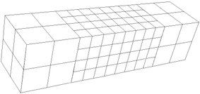
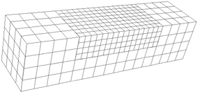
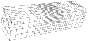
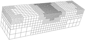
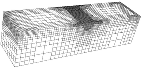
As for the graphical output, the grids generated during the solution look as follow:
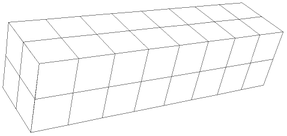
| 
|
| 
|
| 
|
Again, they show essentially the location of singularities introduced by boundary conditions. The vector field computed makes for an interesting graph:
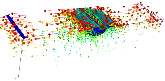
The isocontours shown here as well are those of the pressure variable, showing the singularity at the point of discontinuous velocity boundary conditions.
As explained during the generation of the sparsity pattern, it is important to have the numbering of degrees of freedom in mind when using preconditioners like incomplete LU decompositions. This is most conveniently visualized using the distribution of nonzero elements in the stiffness matrix.
If we don't do anything special to renumber degrees of freedom (i.e., without using DoFRenumbering::Cuthill_McKee, but with using DoFRenumbering::component_wise to ensure that degrees of freedom are appropriately sorted into their corresponding blocks of the matrix and vector), then we get the following image after the first adaptive refinement in two dimensions:
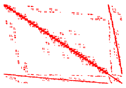
In order to generate such a graph, you have to insert a piece of code like the following to the end of the setup step.
It is clearly visible that the nonzero entries are spread over almost the whole matrix. This makes preconditioning by ILU inefficient: ILU generates a Gaussian elimination (LU decomposition) without fill-in elements, which means that more tentative fill-ins left out will result in a worse approximation of the complete decomposition.
In this program, we have thus chosen a more advanced renumbering of components. The renumbering with DoFRenumbering::Cuthill_McKee and grouping the components into velocity and pressure yields the following output:
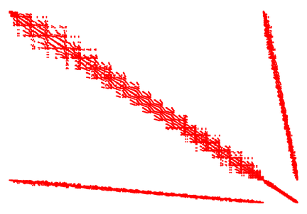
It is apparent that the situation has improved a lot. Most of the elements are now concentrated around the diagonal in the (0,0) block in the matrix. Similar effects are also visible for the other blocks. In this case, the ILU decomposition will be much closer to the full LU decomposition, which improves the quality of the preconditioner. (It may be interesting to note that the sparse direct solver UMFPACK does some internal renumbering of the equations before actually generating a sparse LU decomposition; that procedure leads to a very similar pattern to the one we got from the Cuthill-McKee algorithm.)
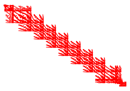
Finally, we want to have a closer look at a sparsity pattern in 3D. We show only the (0,0) block of the matrix, again after one adaptive refinement. Apart from the fact that the matrix size has increased, it is also visible that there are many more entries in the matrix. Moreover, even for the optimized renumbering, there will be a considerable amount of tentative fill-in elements. This illustrates why UMFPACK is not a good choice in 3D - a full decomposition needs many new entries that eventually won't fit into the physical memory (RAM):
We have seen in the section of computational results that the number of outer iterations does not depend on the mesh size, which is optimal in a sense of scalability. This does, however, not apply to the solver as a whole, as mentioned above: We did not look at the number of inner iterations when generating the inverse of the matrix A and the mass matrix M_p. Of course, this is unproblematic in the 2D case where we precondition A with a direct solver and the vmult operation of the inverse matrix structure will converge in one single CG step, but this changes in 3D where we only use an ILU preconditioner. There, the number of required preconditioned CG steps to invert A increases as the mesh is refined, and each vmult operation involves on average approximately 14, 23, 36, 59, 75 and 101 inner CG iterations in the refinement steps shown above. (On the other hand, the number of iterations for applying the inverse pressure mass matrix is always around five, both in two and three dimensions.) To summarize, most work is spent on solving linear systems with the same matrix A over and over again. What makes this look even worse is the fact that we actually invert a matrix that is about 95 percent the size of the total system matrix and stands for 85 percent of the non-zero entries in the sparsity pattern. Hence, the natural question is whether it is reasonable to solve a linear system with matrix A for about 15 times when calculating the solution to the block system.
The answer is, of course, that we can do that in a few other (most of the time better) ways. Nevertheless, it has to be remarked that an indefinite system as the one at hand puts indeed much higher demands on the linear algebra than standard elliptic problems as we have seen in the early tutorial programs. The improvements are still rather unsatisfactory, if one compares with an elliptic problem of similar size. Either way, we will introduce below a number of improvements to the linear solver, a discussion that we will re-consider again with additional options in the step-31 program.
A first attempt to improve the speed of the linear solution process is to choose a dof reordering that makes the ILU being closer to a full LU decomposition, as already mentioned in the in-code comments. The DoFRenumbering namespace compares several choices for the renumbering of dofs for the Stokes equations. The best result regarding the computing time was found for the King ordering, which is accessed through the call DoFRenumbering::boost::king_ordering. With that program, the inner solver needs considerably less operations, e.g. about 62 inner CG iterations for the inversion of A at cycle 4 compared to about 75 iterations with the standard Cuthill-McKee-algorithm. Also, the computing time at cycle 4 decreased from about 17 to 11 minutes for the solve() call. However, the King ordering (and the orderings provided by the DoFRenumbering::boost namespace in general) has a serious drawback - it uses much more memory than the in-build deal versions, since it acts on abstract graphs rather than the geometry provided by the triangulation. In the present case, the renumbering takes about 5 times as much memory, which yields an infeasible algorithm for the last cycle in 3D with 1.2 million unknowns.
Another idea to improve the situation even more would be to choose a preconditioner that makes CG for the (0,0) matrix A converge in a mesh-independent number of iterations, say 10 to 30. We have seen such a candidate in step-16: multigrid.
Even with a good preconditioner for A, we still need to solve of the same linear system repeatedly (with different right hand sides, though) in order to make the Schur complement solve converge. The approach we are going to discuss here is how inner iteration and outer iteration can be combined. If we persist in calculating the Schur complement, there is no other possibility.
The alternative is to attack the block system at once and use an approximate Schur complement as efficient preconditioner. The idea is as follows: If we find a block preconditioner P such that the matrix
\begin{eqnarray*} P^{-1}\left(\begin{array}{cc} A & B^T \\ B & 0 \end{array}\right) \end{eqnarray*}
is simple, then an iterative solver with that preconditioner will converge in a few iterations. Using the Schur complement S = B A^{-1} B^T, one finds that
\begin{eqnarray*} P^{-1} = \left(\begin{array}{cc} A^{-1} & 0 \\ S^{-1} B A^{-1} & -S^{-1} \end{array}\right) \end{eqnarray*}
would appear to be a good choice since
\begin{eqnarray*} P^{-1}\left(\begin{array}{cc} A & B^T \\ B & 0 \end{array}\right) = \left(\begin{array}{cc} A^{-1} & 0 \\ S^{-1} B A^{-1} & -S^{-1} \end{array}\right)\cdot \left(\begin{array}{cc} A & B^T \\ B & 0 \end{array}\right) = \left(\begin{array}{cc} I & A^{-1} B^T \\ 0 & I \end{array}\right). \end{eqnarray*}
This is the approach taken by the paper by Silvester and Wathen referenced to in the introduction (with the exception that Silvester and Wathen use right preconditioning). In this case, a Krylov-based iterative method would converge in one step only if exact inverses of A and S were applied, since all the eigenvalues are one (and the number of iterations in such a method is bounded by the number of distinct eigenvalues). Below, we will discuss the choice of an adequate solver for this problem. First, we are going to have a closer look at the implementation of the preconditioner.
Since P is aimed to be a preconditioner only, we shall use approximations to the inverse of the Schur complement S and the matrix A. Hence, the Schur complement will be approximated by the pressure mass matrix M_p, and we use a preconditioner to A (without an InverseMatrix class around it) for approximating A^{-1}.
Here comes the class that implements the block Schur complement preconditioner. The vmult operation for block vectors according to the derivation above can be specified by three successive operations:
Since we act on the whole block system now, we have to live with one disadvantage: we need to perform the solver iterations on the full block system instead of the smaller pressure space.
Now we turn to the question which solver we should use for the block system. The first observation is that the resulting preconditioned matrix cannot be solved with CG since it is neither positive definite nor symmetric.
The deal.II libraries implement several solvers that are appropriate for the problem at hand. One choice is the solver BiCGStab, which was used for the solution of the unsymmetric advection problem in step-9. The second option, the one we are going to choose, is GMRES (generalized minimum residual). Both methods have their pros and cons - there are problems where one of the two candidates clearly outperforms the other, and vice versa. Wikipedia's article on the GMRES method gives a comparative presentation. A more comprehensive and well-founded comparison can be read e.g. in the book by J.W. Demmel (Applied Numerical Linear Algebra, SIAM, 1997, section 6.6.6).
For our specific problem with the ILU preconditioner for A, we certainly need to perform hundreds of iterations on the block system for large problem sizes (we won't beat CG!). Actually, this disfavors GMRES: During the GMRES iterations, a basis of Krylov vectors is successively built up and some operations are performed on these vectors. The more vectors are in this basis, the more operations and memory will be needed. The number of operations scales as {\cal O}(n + k^2) and memory as {\cal O}(kn), where k is the number of vectors in the Krylov basis and n the size of the (block) matrix. To not let these demands grow excessively, deal.II limits the size k of the basis to 30 vectors by default. Then, the basis is rebuilt. This implementation of the GMRES method is called GMRES(k), with default k=30. What we have gained by this restriction, namely a bound on operations and memory requirements, will be compensated by the fact that we use an incomplete basis - this will increase the number of required iterations.
BiCGStab, on the other hand, won't get slower when many iterations are needed (one iteration uses only results from one preceding step and not all the steps as GMRES). Besides the fact the BiCGStab is more expensive per step since two matrix-vector products are needed (compared to one for CG or GMRES), there is one main reason which makes BiCGStab not appropriate for this problem: The preconditioner applies the inverse of the pressure mass matrix by using the InverseMatrix class. Since the application of the inverse matrix to a vector is done only in approximative way (an exact inverse is too expensive), this will also affect the solver. In the case of BiCGStab, the Krylov vectors will not be orthogonal due to that perturbation. While this is uncritical for a small number of steps (up to about 50), it ruins the performance of the solver when these perturbations have grown to a significant magnitude in the coarse of iterations.
We did some experiments with BiCGStab and found it to be faster than GMRES up to refinement cycle 3 (in 3D), but it became very slow for cycles 4 and 5 (even slower than the original Schur complement), so the solver is useless in this situation. Choosing a sharper tolerance for the inverse matrix class (1e-10*src.l2_norm() instead of 1e-6*src.l2_norm()) made BiCGStab perform well also for cycle 4, but did not change the failure on the very large problems.
GMRES is of course also effected by the approximate inverses, but it is not as sensitive to orthogonality and retains a relatively good performance also for large sizes, see the results below.
With this said, we turn to the realization of the solver call with GMRES with k=100 temporary vectors:
Obviously, one needs to add the include file <lac/solver_gmres.h> in order to make this run. We call the solver with a BlockVector template in order to enable GMRES to operate on block vectors and matrices. Note also that we need to set the (1,1) block in the system matrix to zero (we saved the pressure mass matrix there which is not part of the problem) after we copied the information to another matrix.
Using the Timer class, we collect some statistics that compare the runtime of the block solver with the one from the problem implementation above. Besides the solution with the two options we also check if the solutions of the two variants are close to each other (i.e. this solver gives indeed the same solution as we had before) and calculate the infinity norm of the vector difference.
Let's first see the results in 2D:
We see that there is no huge difference in the solution time between the block Schur complement preconditioner solver and the Schur complement itself. The reason is simple: we used a direct solve as preconditioner for A - so we cannot expect any gain by avoiding the inner iterations. We see that the number of iterations has slightly increased for GMRES, but all in all the two choices are fairly similar.
The picture of course changes in 3D:
Here, the block preconditioned solver is clearly superior to the Schur complement, but the advantage gets less for more mesh points. This is because GMRES(k) scales worse with the problem size than CG, as we discussed above. Nonetheless, the improvement by a factor of 3-6 for moderate problem sizes is quite impressive.
An ultimate linear solver for this problem could be imagined as a combination of an optimal preconditioner for A (e.g. multigrid) and the block preconditioner described above, which is the approach taken in the step-31 and step-32 tutorial programs (where we use an algebraic multigrid method) and step-56 (where we use a geometric multigrid method).
Another possibility that can be taken into account is to not set up a block system, but rather solve the system of velocity and pressure all at once. The options are direct solve with UMFPACK (2D) or GMRES with ILU preconditioning (3D). It should be straightforward to try that.
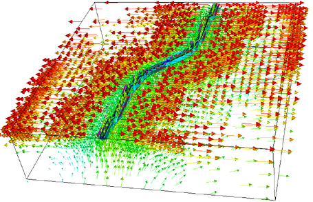
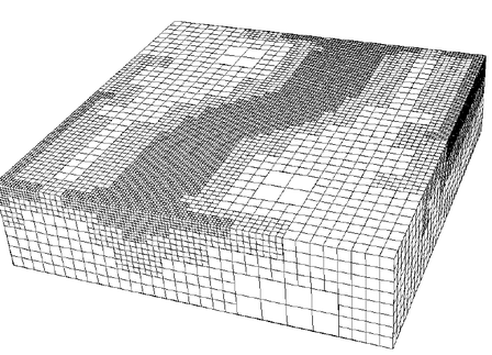
The program can of course also serve as a basis to compute the flow in more interesting cases. The original motivation to write this program was for it to be a starting point for some geophysical flow problems, such as the movement of magma under places where continental plates drift apart (for example mid-ocean ridges). Of course, in such places, the geometry is more complicated than the examples shown above, but it is not hard to accommodate for that.
For example, by using the following modification of the boundary values function
and the following way to generate the mesh as the domain [-2,2]\times[-2,2]\times[-1,0]
then we get images where the fault line is curved:
| 
|
 1.8.14