 |
Reference documentation for deal.II version 9.1.1
|
 |
Reference documentation for deal.II version 9.1.1
|
This tutorial depends on step-6.
| Table of contents | |
|---|---|
| |
This tutorial program attempts to show how to use \(hp\) finite element methods with deal.II. It solves the Laplace equation and so builds only on the first few tutorial programs, in particular on step-4 for dimension independent programming and step-6 for adaptive mesh refinement.
The \(hp\) finite element method was proposed in the early 1980s by Babuska and Guo as an alternative to either (i) mesh refinement (i.e. decreasing the mesh parameter \(h\) in a finite element computation) or (ii) increasing the polynomial degree \(p\) used for shape functions. It is based on the observation that increasing the polynomial degree of the shape functions reduces the approximation error if the solution is sufficiently smooth. On the other hand, it is well known that even for the generally well-behaved class of elliptic problems, higher degrees of regularity can not be guaranteed in the vicinity of boundaries, corners, or where coefficients are discontinuous; consequently, the approximation can not be improved in these areas by increasing the polynomial degree \(p\) but only by refining the mesh, i.e., by reducing the mesh size \(h\). These differing means to reduce the error have led to the notion of \(hp\) finite elements, where the approximating finite element spaces are adapted to have a high polynomial degree \(p\) wherever the solution is sufficiently smooth, while the mesh width \(h\) is reduced at places wherever the solution lacks regularity. It was already realized in the first papers on this method that \(hp\) finite elements can be a powerful tool that can guarantee that the error is reduced not only with some negative power of the number of degrees of freedom, but in fact exponentially.
In order to implement this method, we need several things above and beyond what a usual finite element program needs, and in particular above what we have introduced in the tutorial programs leading up to step-6. In particular, we will have to discuss the following aspects:
Instead of using the same finite element on all cells, we now will want a collection of finite element objects, and associate each cell with one of these objects in this collection.
Degrees of freedom will then have to be allocated on each cell depending on what finite element is associated with this particular cell. Constraints will have to generated in the same way as for hanging nodes, but now also including the case where two neighboring cells.
We will need to be able to assemble cell and face contributions to global matrices and right hand side vectors.
We will discuss all these aspects in the following subsections of this introduction. It will not come as a big surprise that most of these tasks are already well supported by functionality provided by the deal.II, and that we will only have to provide the logic of what the program should do, not exactly how all this is going to happen.
In deal.II, the \(hp\) functionality is largely packaged into the hp namespace. This namespace provides classes that handle \(hp\) discretizations, assembling matrices and vectors, and other tasks. We will get to know many of them further down below. In addition, most of the functions in the DoFTools, and VectorTools namespaces accept \(hp\) objects in addition to the non- \(hp\) ones. Much of the \(hp\) implementation is also discussed in the hp finite element support documentation module and the links found there.
It may be worth giving a slightly larger perspective at the end of this first part of the introduction. \(hp\) functionality has been implemented in a number of different finite element packages (see, for example, the list of references cited in the hp paper). However, by and large, most of these packages have implemented it only for the (i) the 2d case, and/or (ii) the discontinuous Galerkin method. The latter is a significant simplification because discontinuous finite elements by definition do not require continuity across faces between cells and therefore do not require the special treatment otherwise necessary whenever finite elements of different polynomial degree meet at a common face. In contrast, deal.II implements the most general case, i.e. it allows for continuous and discontinuous elements in 1d, 2d, and 3d, and automatically handles the resulting complexity. In particular, it handles computing the constraints (similar to hanging node constraints) of elements of different degree meeting at a face or edge. The many algorithmic and data structure techniques necessary for this are described in the hp paper for those interested in such detail.
We hope that providing such a general implementation will help explore the potential of \(hp\) methods further.
Now on again to the details of how to use the \(hp\) functionality in deal.II. The first aspect we have to deal with is that now we do not have only a single finite element any more that is used on all cells, but a number of different elements that cells can choose to use. For this, deal.II introduces the concept of a finite element collection, implemented in the class hp::FECollection. In essence, such a collection acts like an object of type std::vector<FiniteElement>, but with a few more bells and whistles and a memory management better suited to the task at hand. As we will later see, we will also use similar quadrature collections, and — although we don't use them here — there is also the concept of mapping collections. All of these classes are described in the hp Collections overview.
In this tutorial program, we will use continuous Lagrange elements of orders 2 through 7 (in 2d) or 2 through 5 (in 3d). The collection of used elements can then be created as follows:
The next task we have to consider is what to do with the list of finite element objects we want to use. In previous tutorial programs, starting with step-2, we have seen that the DoFHandler class is responsible for making the connection between a mesh (described by a Triangulation object) and a finite element, by allocating the correct number of degrees of freedom for each vertex, face, edge, and cell of the mesh.
The situation here is a bit more complicated since we do not just have a single finite element object, but rather may want to use different elements on different cells. We therefore need two things: (i) a version of the DoFHandler class that can deal with this situation, and (ii) a way to tell the DoF handler which element to use on which cell.
The first of these two things is implemented in the hp::DoFHandler class: rather than associating it with a triangulation and a single finite element object, it is associated with a triangulation and a finite element collection. The second part is achieved by a loop over all cells of this hp::DoFHandler and for each cell setting the index of the finite element within the collection that shall be used on this cell. We call the index of the finite element object within the collection that shall be used on a cell the cell's active FE index to indicate that this is the finite element that is active on this cell, whereas all the other elements of the collection are inactive on it. The general outline of this reads like this:
Dots in the call to set_active_fe_index() indicate that we will have to have some sort of strategy later on to decide which element to use on which cell; we will come back to this later. The main point here is that the first and last line of this code snippet is pretty much exactly the same as for the non- \(hp\) case.
Another complication arises from the fact that this time we do not simply have hanging nodes from local mesh refinement, but we also have to deal with the case that if there are two cells with different active finite element indices meeting at a face (for example a Q2 and a Q3 element) then we have to compute additional constraints on the finite element field to ensure that it is continuous. This is conceptually very similar to how we compute hanging node constraints, and in fact the code looks exactly the same:
In other words, the DoFTools::make_hanging_node_constraints deals not only with hanging node constraints, but also with \(hp\) constraints at the same time.
Following this, we have to set up matrices and vectors for the linear system of the correct size and assemble them. Setting them up works in exactly the same way as for the non- \(hp\) case. Assembling requires a bit more thought.
The main idea is of course unchanged: we have to loop over all cells, assemble local contributions, and then copy them into the global objects. As discussed in some detail first in step-3, deal.II has the FEValues class that pulls the finite element description, mapping, and quadrature formula together and aids in evaluating values and gradients of shape functions as well as other information on each of the quadrature points mapped to the real location of a cell. Every time we move on to a new cell we re-initialize this FEValues object, thereby asking it to re-compute that part of the information that changes from cell to cell. It can then be used to sum up local contributions to bilinear form and right hand side.
In the context of \(hp\) finite element methods, we have to deal with the fact that we do not use the same finite element object on each cell. In fact, we should not even use the same quadrature object for all cells, but rather higher order quadrature formulas for cells where we use higher order finite elements. Similarly, we may want to use higher order mappings on such cells as well.
To facilitate these considerations, deal.II has a class hp::FEValues that does what we need in the current context. The difference is that instead of a single finite element, quadrature formula, and mapping, it takes collections of these objects. It's use is very much like the regular FEValues class, i.e. the interesting part of the loop over all cells would look like this:
In this tutorial program, we will always use a Q1 mapping, so the mapping collection argument to the hp::FEValues construction will be omitted. Inside the loop, we first initialize the hp::FEValues object for the current cell. The second, third and fourth arguments denote the index within their respective collections of the quadrature, mapping, and finite element objects we wish to use on this cell. These arguments can be omitted (and are in the program below), in which case cell->active_fe_index() is used for this index. The order of these arguments is chosen in this way because one may sometimes want to pick a different quadrature or mapping object from their respective collections, but hardly ever a different finite element than the one in use on this cell, i.e. one with an index different from cell->active_fe_index(). The finite element collection index is therefore the last default argument so that it can be conveniently omitted.
What this reinit call does is the following: the hp::FEValues class checks whether it has previously already allocated a non- \(hp\) FEValues object for this combination of finite element, quadrature, and mapping objects. If not, it allocates one. It then re-initializes this object for the current cell, after which there is now a FEValues object for the selected finite element, quadrature and mapping usable on the current cell. A reference to this object is then obtained using the call hp_fe_values.get_present_fe_values(), and will be used in the usual fashion to assemble local contributions.
One of the central pieces of the adaptive finite element method is that we inspect the computed solution (a posteriori) with an indicator that tells us which are the cells where the error is largest, and then refine them. In many of the other tutorial programs, we use the KellyErrorEstimator class to get an indication of the size of the error on a cell, although we also discuss more complicated strategies in some programs, most importantly in step-14.
In any case, as long as the decision is only "refine this cell" or "do not refine this cell", the actual refinement step is not particularly challenging. However, here we have a code that is capable of hp refinement, i.e. we suddenly have two choices whenever we detect that the error on a certain cell is too large for our liking: we can refine the cell by splitting it into several smaller ones, or we can increase the polynomial degree of the shape functions used on it. How do we know which is the more promising strategy? Answering this question is the central problem in \(hp\) finite element research at the time of this writing.
In short, the question does not appear to be settled in the literature at this time. There are a number of more or less complicated schemes that address it, but there is nothing like the KellyErrorEstimator that is universally accepted as a good, even if not optimal, indicator of the error. Most proposals use the fact that it is beneficial to increase the polynomial degree whenever the solution is locally smooth whereas it is better to refine the mesh wherever it is rough. However, the questions of how to determine the local smoothness of the solution as well as the decision when a solution is smooth enough to allow for an increase in \(p\) are certainly big and important ones.
In the following, we propose a simple estimator of the local smoothness of a solution. As we will see in the results section, this estimator has flaws, in particular as far as cells with local hanging nodes are concerned. We therefore do not intend to present the following ideas as a complete solution to the problem. Rather, it is intended as an idea to approach it that merits further research and investigation. In other words, we do not intend to enter a sophisticated proposal into the fray about answers to the general question. However, to demonstrate our approach to \(hp\) finite elements, we need a simple indicator that does generate some useful information that is able to drive the simple calculations this tutorial program will perform.
Our approach here is simple: for a function \(u({\bf x})\) to be in the Sobolev space \(H^s(K)\) on a cell \(K\), it has to satisfy the condition
\[ \int_K |\nabla^s u({\bf x})|^2 \; d{\bf x} < \infty. \]
Assuming that the cell \(K\) is not degenerate, i.e. that the mapping from the unit cell to cell \(K\) is sufficiently regular, above condition is of course equivalent to
\[ \int_{\hat K} |\nabla^s \hat u(\hat{\bf x})|^2 \; d\hat{\bf x} < \infty\,, \]
where \(\hat u(\hat{\bf x})\) is the function \(u({\bf x})\) mapped back onto the unit cell \(\hat K\). From here, we can do the following: first, let us define the Fourier series of \(\hat u\) as
\[ \hat u(\hat{\bf x}) = \sum_{\bf k} \hat U_{\bf k}\,e^{-i {\bf k}\cdot \hat{\bf x}}, \]
with Fourier vectors \({\bf k}=(k_x,k_y)\) in 2d, \({\bf k}=(k_x,k_y,k_z)\) in 3d, etc, and \(k_x,k_y,k_z=0,2\pi,4\pi,\ldots\). The coefficients of expansion \(\hat U_{\bf k}\) can be obtained using \(L^2\)-orthogonality of the exponential basis
\[ \int_{\hat K} e^{-i {\bf m}\cdot \hat{\bf x}} e^{i {\bf n}\cdot \hat{\bf x}} d\hat{\bf x} = \delta_{\bf m \bf n}, \]
that leads to the following expression
\[ \hat U_{\bf k} = \int_{\hat K} e^{i {\bf k}\cdot \hat{\bf x}} \hat u(\hat{\bf x}) d\hat{\bf x} \,. \]
It becomes clear that we can then write the \(H^s\) norm of \(\hat u\) as
\[ \int_{\hat K} |\nabla^s \hat u(\hat{\bf x})|^2 \; d\hat{\bf x} = \int_{\hat K} \left| \sum_{\bf k} |{\bf k}|^s e^{-i{\bf k}\cdot \hat{\bf x}} \hat U_{\bf k} \right|^2 \; d\hat{\bf x} = \sum_{\bf k} |{\bf k}|^{2s} |\hat U_{\bf k}|^2. \]
In other words, if this norm is to be finite (i.e. for \(\hat u(\hat{\bf x})\) to be in \(H^s(\hat K)\)), we need that
\[ |\hat U_{\bf k}| = {\cal O}\left(|{\bf k}|^{-\left(s+1/2+\frac{d-1}{2}+\epsilon\right)}\right). \]
Put differently: the higher regularity \(s\) we want, the faster the Fourier coefficients have to go to zero. If you wonder where the additional exponent \(\frac{d-1}2\) comes from: we would like to make use of the fact that \(\sum_l a_l < \infty\) if the sequence \(a_l = {\cal O}(l^{-1-\epsilon})\) for any \(\epsilon>0\). The problem is that we here have a summation not only over a single variable, but over all the integer multiples of \(2\pi\) that are located inside the \(d\)-dimensional sphere, because we have vector components \(k_x, k_y, \ldots\). In the same way as we prove that the sequence \(a_l\) above converges by replacing the sum by an integral over the entire line, we can replace our \(d\)-dimensional sum by an integral over \(d\)-dimensional space. Now we have to note that between distance \(|{\bf k}|\) and \(|{\bf k}|+d|{\bf k}|\), there are, up to a constant, \(|{\bf k}|^{d-1}\) modes, in much the same way as we can transform the volume element \(dx\;dy\) into \(2\pi r\; dr\). Consequently, it is no longer \(|{\bf k}|^{2s}|\hat U_{\bf k}|^2\) that has to decay as \({\cal O}(|{\bf k}|^{-1-\epsilon})\), but it is in fact \(|{\bf k}|^{2s}|\hat U_{\bf k}|^2 |{\bf k}|^{d-1}\). A comparison of exponents yields the result.
We can turn this around: Assume we are given a function \(\hat u\) of unknown smoothness. Let us compute its Fourier coefficients \(\hat U_{\bf k}\) and see how fast they decay. If they decay as
\[ |\hat U_{\bf k}| = {\cal O}(|{\bf k}|^{-\mu-\epsilon}), \]
then consequently the function we had here was in \(H^{\mu-d/2}\).
So what do we have to do to estimate the local smoothness of \(u({\bf x})\) on a cell \(K\)? Clearly, the first step is to compute the Fourier coefficients of our solution. Fourier series being infinite series, we simplify our task by only computing the first few terms of the series, such that \(|{\bf k}|\le 2\pi N\) with a cut-off \(N\). Let us parenthetically remark that we want to choose \(N\) large enough so that we capture at least the variation of those shape functions that vary the most. On the other hand, we should not choose \(N\) too large: clearly, a finite element function, being a polynomial, is in \(C^\infty\) on any given cell, so the coefficients will have to decay exponentially at one point; since we want to estimate the smoothness of the function this polynomial approximates, not of the polynomial itself, we need to choose a reasonable cutoff for \(N\). Either way, computing this series is not particularly hard: from the definition
\[ \hat U_{\bf k} = \int_{\hat K} e^{i {\bf k}\cdot \hat{\bf x}} \hat u(\hat{\bf x}) d\hat{\bf x} \]
we see that we can compute the coefficient \(\hat U_{\bf k}\) as
\[ \hat U_{\bf k} = \sum_{i=0}^{\textrm{dofs per cell}} \left[\int_{\hat K} e^{i {\bf k}\cdot \hat{\bf x}} \hat \varphi_i(\hat{\bf x}) d\hat{\bf x} \right] u_i, \]
where \(u_i\) is the value of the \(i\)th degree of freedom on this cell. In other words, we can write it as a matrix-vector product
\[ \hat U_{\bf k} = {\cal F}_{{\bf k},j} u_j, \]
with the matrix
\[ {\cal F}_{{\bf k},j} = \int_{\hat K} e^{i {\bf k}\cdot \hat{\bf x}} \hat \varphi_j(\hat{\bf x}) d\hat{\bf x}. \]
This matrix is easily computed for a given number of shape functions \(\varphi_j\) and Fourier modes \(N\). Consequently, finding the coefficients \(\hat U_{\bf k}\) is a rather trivial job. To simplify our life even further, we will use FESeries::Fourier class which does exactly this.
The next task is that we have to estimate how fast these coefficients decay with \(|{\bf k}|\). The problem is that, of course, we have only finitely many of these coefficients in the first place. In other words, the best we can do is to fit a function \(\alpha |{\bf k}|^{-\mu}\) to our data points \(\hat U_{\bf k}\), for example by determining \(\alpha,\mu\) via a least-squares procedure:
\[ \min_{\alpha,\mu} \frac 12 \sum_{{\bf k}, |{\bf k}|\le N} \left( |\hat U_{\bf k}| - \alpha |{\bf k}|^{-\mu}\right)^2 \]
However, the problem with this is that it leads to a nonlinear problem, a fact that we would like to avoid. On the other hand, we can transform the problem into a simpler one if we try to fit the logarithm of our coefficients to the logarithm of \(\alpha |{\bf k}|^{-\mu}\), like this:
\[ \min_{\alpha,\mu} Q(\alpha,\mu) = \frac 12 \sum_{{\bf k}, |{\bf k}|\le N} \left( \ln |\hat U_{\bf k}| - \ln (\alpha |{\bf k}|^{-\mu})\right)^2. \]
Using the usual facts about logarithms, we see that this yields the problem
\[ \min_{\beta,\mu} Q(\beta,\mu) = \frac 12 \sum_{{\bf k}, |{\bf k}|\le N} \left( \ln |\hat U_{\bf k}| - \beta + \mu \ln |{\bf k}|\right)^2, \]
where \(\beta=\ln \alpha\). This is now a problem for which the optimality conditions \(\frac{\partial Q}{\partial\beta}=0, \frac{\partial Q}{\partial\mu}=0\), are linear in \(\beta,\mu\). We can write these conditions as follows:
\[ \left(\begin{array}{cc} \sum_{{\bf k}, |{\bf k}|\le N} 1 & \sum_{{\bf k}, |{\bf k}|\le N} \ln |{\bf k}| \\ \sum_{{\bf k}, |{\bf k}|\le N} \ln |{\bf k}| & \sum_{{\bf k}, |{\bf k}|\le N} (\ln |{\bf k}|)^2 \end{array}\right) \left(\begin{array}{c} \beta \\ -\mu \end{array}\right) = \left(\begin{array}{c} \sum_{{\bf k}, |{\bf k}|\le N} \ln |\hat U_{{\bf k}}| \\ \sum_{{\bf k}, |{\bf k}|\le N} \ln |\hat U_{{\bf k}}| \ln |{\bf k}| \end{array}\right) \]
This linear system is readily inverted to yield
\[ \beta = \frac { \left(\sum_{{\bf k}, |{\bf k}|\le N} (\ln |{\bf k}|)^2\right) \left(\sum_{{\bf k}, |{\bf k}|\le N} \ln |\hat U_{{\bf k}}|\right) - \left(\sum_{{\bf k}, |{\bf k}|\le N} \ln |{\bf k}|\right) \left(\sum_{{\bf k}, |{\bf k}|\le N} \ln |\hat U_{{\bf k}}| \ln |{\bf k}| \right) } { \left(\sum_{{\bf k}, |{\bf k}|\le N} 1\right) \left(\sum_{{\bf k}, |{\bf k}|\le N} (\ln |{\bf k}|)^2\right) - \left(\sum_{{\bf k}, |{\bf k}|\le N} \ln |{\bf k}|\right)^2 } \]
and
\[ \mu = \frac { \left(\sum_{{\bf k}, |{\bf k}|\le N} \ln |{\bf k}|\right) \left(\sum_{{\bf k}, |{\bf k}|\le N} \ln |\hat U_{{\bf k}}|\right) - \left(\sum_{{\bf k}, |{\bf k}|\le N} 1\right) \left(\sum_{{\bf k}, |{\bf k}|\le N} \ln |\hat U_{{\bf k}}| \ln |{\bf k}| \right) } { \left(\sum_{{\bf k}, |{\bf k}|\le N} 1\right) \left(\sum_{{\bf k}, |{\bf k}|\le N} (\ln |{\bf k}|)^2\right) - \left(\sum_{{\bf k}, |{\bf k}|\le N} \ln |{\bf k}|\right)^2 }. \]
This is nothing else but linear regression fit and to do that we will use FESeries::linear_regression(). While we are not particularly interested in the actual value of \(\beta\), the formula above gives us a mean to calculate the value of the exponent \(\mu\) that we can then use to determine that \(\hat u(\hat{\bf x})\) is in \(H^s(\hat K)\) with \(s=\mu-\frac d2\).
In the formulas above, we have derived the Fourier coefficients \(\hat U_{\bf k}\). Because \({\bf k}\) is a vector, we will get a number of Fourier coefficients \(\hat U_{{\bf k}}\) for the same absolute value \(|{\bf k}|\), corresponding to the Fourier transform in different directions. If we now consider a function like \(|x|y^2\) then we will find lots of large Fourier coefficients in \(x\)-direction because the function is non-smooth in this direction, but fast-decaying Fourier coefficients in \(y\)-direction because the function is smooth there. The question that arises is this: if we simply fit our polynomial decay \(\alpha |{\bf k}|^\mu\) to all Fourier coefficients, we will fit it to a smoothness averaged in all spatial directions. Is this what we want? Or would it be better to only consider the largest coefficient \(\hat U_{{\bf k}}\) for all \({\bf k}\) with the same magnitude, essentially trying to determine the smoothness of the solution in that spatial direction in which the solution appears to be roughest?
One can probably argue for either case. The issue would be of more interest if deal.II had the ability to use anisotropic finite elements, i.e. ones that use different polynomial degrees in different spatial directions, as they would be able to exploit the directionally variable smoothness much better. Alas, this capability does not exist at the time of writing this tutorial program.
Either way, because we only have isotopic finite element classes, we adopt the viewpoint that we should tailor the polynomial degree to the lowest amount of regularity, in order to keep numerical efforts low. Consequently, instead of using the formula
\[ \mu = \frac { \left(\sum_{{\bf k}, |{\bf k}|\le N} \ln |{\bf k}|\right) \left(\sum_{{\bf k}, |{\bf k}|\le N} \ln |\hat U_{{\bf k}}|\right) - \left(\sum_{{\bf k}, |{\bf k}|\le N} 1\right) \left(\sum_{{\bf k}, |{\bf k}|\le N} \ln |\hat U_{{\bf k}}| \ln |{\bf k}| \right) } { \left(\sum_{{\bf k}, |{\bf k}|\le N} 1\right) \left(\sum_{{\bf k}, |{\bf k}|\le N} (\ln |{\bf k}|)^2\right) - \left(\sum_{{\bf k}, |{\bf k}|\le N} \ln |{\bf k}|\right)^2 }. \]
To calculate \(\mu\) as shown above, we have to slightly modify all sums: instead of summing over all Fourier modes, we only sum over those for which the Fourier coefficient is the largest one among all \(\hat U_{{\bf k}}\) with the same magnitude \(|{\bf k}|\), i.e. all sums above have to replaced by the following sums:
\[ \sum_{{\bf k}, |{\bf k}|\le N} \longrightarrow \sum_{\begin{matrix}{{\bf k}, |{\bf k}|\le N} \\ {|\hat U_{{\bf k}}| \ge |\hat U_{{\bf k}'}| \ \textrm{for all}\ {\bf k}'\ \textrm{with}\ |{\bf k}'|=|{\bf k}|}\end{matrix}}. \]
This is the form we will implement in the program.
One may ask whether it is a problem that we only compute the Fourier transform on the reference cell (rather than the real cell) of the solution. After all, we stretch the solution by a factor \(\frac 1h\) during the transformation, thereby shifting the Fourier frequencies by a factor of \(h\). This is of particular concern since we may have neighboring cells with mesh sizes \(h\) that differ by a factor of 2 if one of them is more refined than the other. The concern is also motivated by the fact that, as we will see in the results section below, the estimated smoothness of the solution should be a more or less continuous function, but exhibits jumps at locations where the mesh size jumps. It therefore seems natural to ask whether we have to compensate for the transformation.
The short answer is "no". In the process outlined above, we attempt to find coefficients \(\beta,\mu\) that minimize the sum of squares of the terms
\[ \ln |\hat U_{{\bf k}}| - \beta + \mu \ln |{\bf k}|. \]
To compensate for the transformation means not attempting to fit a decay \(|{\bf k}|^\mu\) with respect to the Fourier frequencies \({\bf k}\) on the unit cell, but to fit the coefficients \(\hat U_{{\bf k}}\) computed on the reference cell to the Fourier frequencies on the real cell \(|\bf k|h\), where \(h\) is the norm of the transformation operator (i.e. something like the diameter of the cell). In other words, we would have to minimize the sum of squares of the terms
\[ \ln |\hat U_{{\bf k}}| - \beta + \mu \ln (|{\bf k}|h). \]
instead. However, using fundamental properties of the logarithm, this is simply equivalent to minimizing
\[ \ln |\hat U_{{\bf k}}| - (\beta - \mu \ln h) + \mu \ln (|{\bf k}|). \]
In other words, this and the original least squares problem will produce the same best-fit exponent \(\mu\), though the offset will in one case be \(\beta\) and in the other \(\beta-\mu \ln h\). However, since we are not interested in the offset at all but only in the exponent, it doesn't matter whether we scale Fourier frequencies in order to account for mesh size effects or not, the estimated smoothness exponent will be the same in either case.
One of the problems with \(hp\) methods is that the high polynomial degree of shape functions together with the large number of constrained degrees of freedom leads to matrices with large numbers of nonzero entries in some rows. At the same time, because there are areas where we use low polynomial degree and consequently matrix rows with relatively few nonzero entries. Consequently, allocating the sparsity pattern for these matrices is a challenge: we cannot simply assemble a SparsityPattern by starting with an estimate of the bandwidth without using a lot of extra memory.
The way in which we create a SparsityPattern for the underlying linear system is tightly coupled to the strategy we use to enforce constraints. deal.II supports handling constraints in linear systems in two ways:
Most programs built on deal.II use the DoFTools::make_sparsity_pattern function to allocate a DynamicSparsityPattern that takes constraints into account. The system matrix then uses a SparsityPattern copied over from the DynamicSparsityPattern. This method is explained in step-2 and used in most tutorial programs.
The early tutorial programs use first or second degree finite elements, so removing entries in the sparsity pattern corresponding to constrained degrees of freedom does not have a large impact on the overall number of zeros explicitly stored by the matrix. However, since as many as a third of the degrees of freedom may be constrained in an hp discretization (and, with higher degree elements, these constraints can couple one DoF to as many as ten or twenty other DoFs), it is worthwhile to take these constraints into consideration since the resulting matrix will be much sparser (and, therefore, matrix-vector products or factorizations will be substantially faster too).
A second problem particular to \(hp\) methods arises because we have so many constrained degrees of freedom: typically up to about one third of all degrees of freedom (in 3d) are constrained because they either belong to cells with hanging nodes or because they are on cells adjacent to cells with a higher or lower polynomial degree. This is, in fact, not much more than the fraction of constrained degrees of freedom in non- \(hp\) mode, but the difference is that each constrained hanging node is constrained not only against the two adjacent degrees of freedom, but is constrained against many more degrees of freedom.
It turns out that the strategy presented first in step-6 to eliminate the constraints while computing the element matrices and vectors with AffineConstraints::distribute_local_to_global is the most efficient approach also for this case. The alternative strategy to first build the matrix without constraints and then "condensing" away constrained degrees of freedom is considerably more expensive. It turns out that building the sparsity pattern by this inefficient algorithm requires at least \({\cal O}(N \log N)\) in the number of unknowns, whereas an ideal finite element program would of course only have algorithms that are linear in the number of unknowns. Timing the sparsity pattern creation as well as the matrix assembly shows that the algorithm presented in step-6 (and used in the code below) is indeed faster.
In our program, we will also treat the boundary conditions as (possibly inhomogeneous) constraints and eliminate the matrix rows and columns to those as well. All we have to do for this is to call the function that interpolates the Dirichlet boundary conditions already in the setup phase in order to tell the AffineConstraints object about them, and then do the transfer from local to global data on matrix and vector simultaneously. This is exactly what we've shown in step-6.
The test case we will solve with this program is a re-take of the one we already look at in step-14: we solve the Laplace equation
\[ -\Delta u = f \]
in 2d, with \(f=(x+1)(y+1)\), and with zero Dirichlet boundary values for \(u\). We do so on the domain \([-1,1]^2\backslash[-\frac 12,\frac 12]^2\), i.e. a square with a square hole in the middle.
The difference to step-14 is of course that we use \(hp\) finite elements for the solution. The test case is of interest because it has re-entrant corners in the corners of the hole, at which the solution has singularities. We therefore expect that the solution will be smooth in the interior of the domain, and rough in the vicinity of the singularities. The hope is that our refinement and smoothness indicators will be able to see this behavior and refine the mesh close to the singularities, while the polynomial degree is increased away from it. As we will see in the results section, this is indeed the case.
The first few files have already been covered in previous examples and will thus not be further commented on.
These are the new files we need. The first and second provide hp versions of the DoFHandler and FEValues classes as described in the introduction of this program. The last one provides Fourier transformation class on the unit cell.
The last set of include files are standard C++ headers. We need support for complex numbers when we compute the Fourier transform.
Finally, this is as in previous programs:
The main class of this program looks very much like the one already used in the first few tutorial programs, for example the one in step-6. The main difference is that we have merged the refine_grid and output_results functions into one since we will also want to output some of the quantities used in deciding how to refine the mesh (in particular the estimated smoothness of the solution). There is also a function that computes this estimated smoothness, as discussed in the introduction.
As far as member variables are concerned, we use the same structure as already used in step-6, but instead of a regular DoFHandler we use an object of type hp::DoFHandler, and we need collections instead of individual finite element, quadrature, and face quadrature objects. We will fill these collections in the constructor of the class. The last variable, max_degree, indicates the maximal polynomial degree of shape functions used.
Next, let us define the right hand side function for this problem. It is \(x+1\) in 1d, \((x+1)(y+1)\) in 2d, and so on.
The constructor of this class is fairly straightforward. It associates the hp::DoFHandler object with the triangulation, and then sets the maximal polynomial degree to 7 (in 1d and 2d) or 5 (in 3d and higher). We do so because using higher order polynomial degrees becomes prohibitively expensive, especially in higher space dimensions.
Following this, we fill the collections of finite element, and cell and face quadrature objects. We start with quadratic elements, and each quadrature formula is chosen so that it is appropriate for the matching finite element in the hp::FECollection object.
Finally, we initialize FESeries::Fourier object which will be used to calculate coefficient in Fourier series as described in the introduction. In addition to the hp::FECollection, we need to provide quadrature rules hp::QCollection for integration on the reference cell.
In order to resize fourier_coefficients Table, we use the following auxiliary function
As described in the introduction, we define the Fourier vectors \({\bf k}\) for which we want to compute Fourier coefficients of the solution on each cell as follows. In 2d, we will need coefficients corresponding to vectors \({\bf k}=(2 \pi i, 2\pi j)^T\) for which \(\sqrt{i^2+j^2}\le N\), with \(i,j\) integers and \(N\) being the maximal polynomial degree we use for the finite elements in this program. The FESeries::Fourier class' constructor first parameter \(N\) defines the number of coefficients in 1D with the total number of coefficients being \(N^{dim}\). Although we will not use coefficients corresponding to \(\sqrt{i^2+j^2}> N\) and \(i+j==0\), the overhead of their calculation is minimal. The transformation matrices for each FiniteElement will be calculated only once the first time they are required in the course of hp-adaptive refinement. Because we work on the unit cell, we can do all this work without a mapping from reference to real cell and consequently can precalculate these matrices. The calculation of expansion coefficients for a particular set of local degrees of freedom on a given cell then follows as a simple matrix-vector product. The 3d case is handled analogously.
We will need to assemble the matrices that do the Fourier transforms for each of the finite elements we deal with, i.e. the matrices \({\cal F}_{{\bf k},j}\) defined in the introduction. We have to do that for each of the finite elements in use. To that end we need a quadrature rule. In this example we use the same quadrature formula for each finite element, namely that is obtained by iterating a 2-point Gauss formula as many times as the maximal exponent we use for the term \(e^{i{\bf k}\cdot{\bf x}}\):
Now we are ready to set-up the FESeries::Fourier object
We need to resize the matrix of fourier coefficients according to the number of modes N.
The destructor is unchanged from what we already did in step-6:
This function is again a verbatim copy of what we already did in step-6. Despite function calls with exactly the same names and arguments, the algorithms used internally are different in some aspect since the dof_handler variable here is an hp object.
This is the function that assembles the global matrix and right hand side vector from the local contributions of each cell. Its main working is as has been described in many of the tutorial programs before. The significant deviations are the ones necessary for hp finite element methods. In particular, that we need to use a collection of FEValues object (implemented through the hp::FEValues class), and that we have to eliminate constrained degrees of freedom already when copying local contributions into global objects. Both of these are explained in detail in the introduction of this program.
One other slight complication is the fact that because we use different polynomial degrees on different cells, the matrices and vectors holding local contributions do not have the same size on all cells. At the beginning of the loop over all cells, we therefore each time have to resize them to the correct size (given by dofs_per_cell). Because these classes are implement in such a way that reducing the size of a matrix or vector does not release the currently allocated memory (unless the new size is zero), the process of resizing at the beginning of the loop will only require re-allocation of memory during the first few iterations. Once we have found in a cell with the maximal finite element degree, no more re-allocations will happen because all subsequent reinit calls will only set the size to something that fits the currently allocated memory. This is important since allocating memory is expensive, and doing so every time we visit a new cell would take significant compute time.
The function solving the linear system is entirely unchanged from previous examples. We simply try to reduce the initial residual (which equals the \(l_2\) norm of the right hand side) by a certain factor:
After solving the linear system, we will want to postprocess the solution. Here, all we do is to estimate the error, estimate the local smoothness of the solution as described in the introduction, then write graphical output, and finally refine the mesh in both \(h\) and \(p\) according to the indicators computed before. We do all this in the same function because we want the estimated error and smoothness indicators not only for refinement, but also include them in the graphical output.
Let us start with computing estimated error and smoothness indicators, which each are one number for each active cell of our triangulation. For the error indicator, we use the KellyErrorEstimator class as always. Estimating the smoothness is done in the respective function of this class; that function is discussed further down below:
Next we want to generate graphical output. In addition to the two estimated quantities derived above, we would also like to output the polynomial degree of the finite elements used on each of the elements on the mesh.
The way to do that requires that we loop over all cells and poll the active finite element index of them using cell->active_fe_index(). We then use the result of this operation and query the finite element collection for the finite element with that index, and finally determine the polynomial degree of that element. The result we put into a vector with one element per cell. The DataOut class requires this to be a vector of float or double, even though our values are all integers, so that it what we use:
With now all data vectors available – solution, estimated errors and smoothness indicators, and finite element degrees –, we create a DataOut object for graphical output and attach all data. Note that the DataOut class has a second template argument (which defaults to DoFHandler<dim>, which is why we have never seen it in previous tutorial programs) that indicates the type of DoF handler to be used. Here, we have to use the hp::DoFHandler class:
The final step in generating output is to determine a file name, open the file, and write the data into it (here, we use VTK format):
After this, we would like to actually refine the mesh, in both \(h\) and \(p\). The way we are going to do this is as follows: first, we use the estimated error to flag those cells for refinement that have the largest error. This is what we have always done:
Next we would like to figure out which of the cells that have been flagged for refinement should actually have \(p\) increased instead of \(h\) decreased. The strategy we choose here is that we look at the smoothness indicators of those cells that are flagged for refinement, and increase \(p\) for those with a smoothness larger than a certain threshold. For this, we first have to determine the maximal and minimal values of the smoothness indicators of all flagged cells, which we do using a loop over all cells and comparing current minimal and maximal values. (We start with the minimal and maximal values of all cells, a range within which the minimal and maximal values on cells flagged for refinement must surely lie.) Absent any better strategies, we will then set the threshold above which will increase \(p\) instead of reducing \(h\) as the mean value between minimal and maximal smoothness indicators on cells flagged for refinement:
With this, we can go back, loop over all cells again, and for those cells for which (i) the refinement flag is set, (ii) the smoothness indicator is larger than the threshold, and (iii) we still have a finite element with a polynomial degree higher than the current one in the finite element collection, we then increase the polynomial degree and in return remove the flag indicating that the cell should undergo bisection. For all other cells, the refinement flags remain untouched:
At the end of this procedure, we then refine the mesh. During this process, children of cells undergoing bisection inherit their mother cell's finite element index:
The following function is used when creating the initial grid. It is a specialization for the 2d case, i.e. a corresponding function needs to be implemented if the program is run in anything other then 2d. The function is actually stolen from step-14 and generates the same mesh used already there, i.e. the square domain with the square hole in the middle. The meaning of the different parts of this function are explained in the documentation of step-14:
This function implements the logic of the program, as did the respective function in most of the previous programs already, see for example step-6.
Basically, it contains the adaptive loop: in the first iteration create a coarse grid, and then set up the linear system, assemble it, solve, and postprocess the solution including mesh refinement. Then start over again. In the meantime, also output some information for those staring at the screen trying to figure out what the program does:
As described in the introduction, we will need to take the maximum absolute value of fourier coefficients which correspond to \(k\)-vector \(|{\bf k}|= const\). To filter the coefficients Table we will use the FESeries::process_coefficients() which requires a predicate to be specified. The predicate should operate on TableIndices and return a pair of bool and unsigned int. The latter is the value of the map from TableIndicies to unsigned int. It is used to define subsets of coefficients from which we search for the one with highest absolute value, i.e. \(l^\infty\)-norm. The bool parameter defines which indices should be used in processing. In the current case we are interested in coefficients which correspond to \(0 < i*i+j*j < N*N\) and \(0 < i*i+j*j+k*k < N*N\) in 2D and 3D, respectively.
This last function of significance implements the algorithm to estimate the smoothness exponent using the algorithms explained in detail in the introduction. We will therefore only comment on those points that are of implementational importance.
Since most of the hard work is done for us in FESeries::Fourier and we set up the object of this class in the constructor, what we are left to do here is apply this class to calculate coefficients and then perform linear regression to fit their decay slope.
First thing to do is to loop over all cells and do our work there, i.e. to locally do the Fourier transform and estimate the decay coefficient. We will use the following array as a scratch array in the loop to store local DoF values:
Then here is the loop:
Inside the loop, we first need to get the values of the local degrees of freedom (which we put into the local_dof_values array after setting it to the right size) and then need to compute the Fourier transform by multiplying this vector with the matrix \({\cal F}\) corresponding to this finite element. This is done by calling FESeries::Fourier::calculate(), that has to be provided with the local_dof_values, cell->active_fe_index() and a Table to store coefficients.
The next thing, as explained in the introduction, is that we wanted to only fit our exponential decay of Fourier coefficients to the largest coefficients for each possible value of \(|{\bf k}|\). To this end, we use FESeries::process_coefficients() to rework coefficients into the desired format. We'll only take those Fourier coefficients with the largest magnitude for a given value of \(|{\bf k}|\) and thereby need to use VectorTools::Linfty_norm:
The first vector in the std::pair will store values of the predicate, that is \(i*i+j*j= const\) or \(i*i+j*j+k*k = const\) in 2D or 3D respectively. This vector will be the same for all the cells so we can calculate logarithms of the corresponding Fourier vectors \(|{\bf k}|\) only once in the whole hp-refinement cycle:
We have to calculate the logarithms of absolute values of coefficients and use it in a linear regression fit to obtain \(\mu\).
The final step is to compute the Sobolev index \(s=\mu-\frac d2\) and store it in the vector of estimated values for each cell:
The main function is again verbatim what we had before: wrap creating and running an object of the main class into a try block and catch whatever exceptions are thrown, thereby producing meaningful output if anything should go wrong:
In this section, we discuss a few results produced from running the current tutorial program. More results, in particular the extension to 3d calculations and determining how much compute time the individual components of the program take, are given in the hp_paper .
When run, this is what the program produces:
The first thing we learn from this is that the number of constrained degrees of freedom is on the order of 20-25% of the total number of degrees of freedom, at least on the later grids when we have elements of relatively high order (in 3d, the fraction of constrained degrees of freedom can be up to 30%). This is, in fact, on the same order of magnitude as for non- \(hp\) discretizations. For example, in the last step of the step-6 program, we have 18353 degrees of freedom, 4432 of which are constrained. The difference is that in the latter program, each constrained hanging node is constrained against only the two adjacent degrees of freedom, whereas in the \(hp\) case, constrained nodes are constrained against many more degrees of freedom. Note also that the current program also includes nodes subject to Dirichlet boundary conditions in the list of constraints. In cycle 0, all the constraints are actually because of boundary conditions.
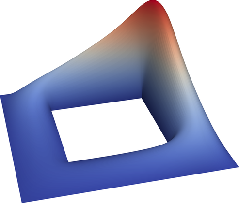
Of maybe more interest is to look at the graphical output. First, here is the solution of the problem:
Secondly, let us look at the sequence of meshes generated:
It is clearly visible how the mesh is refined near the corner singularities, as one would expect it. More interestingly, we should be curious to see the distribution of finite element polynomial degrees to these mesh cells, where grey corresponds to degree two and pink corresponds to degree seven:

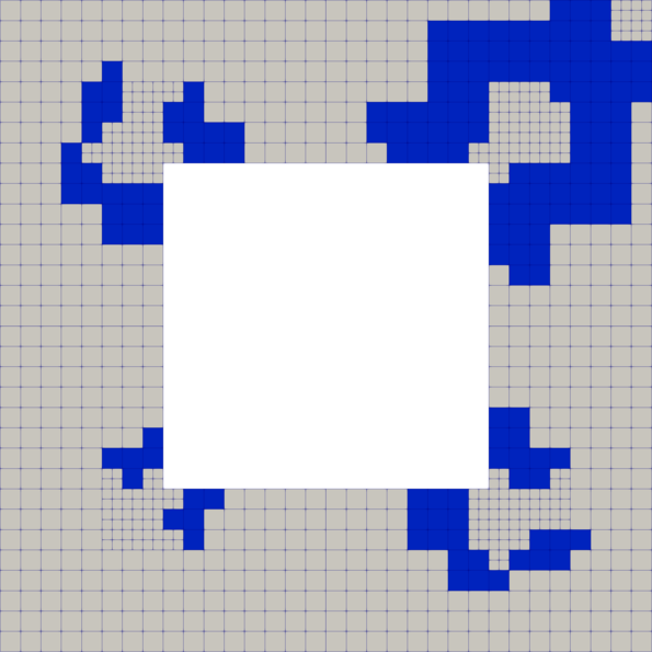
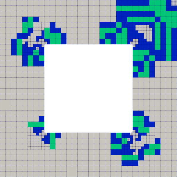

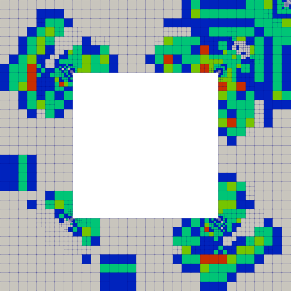
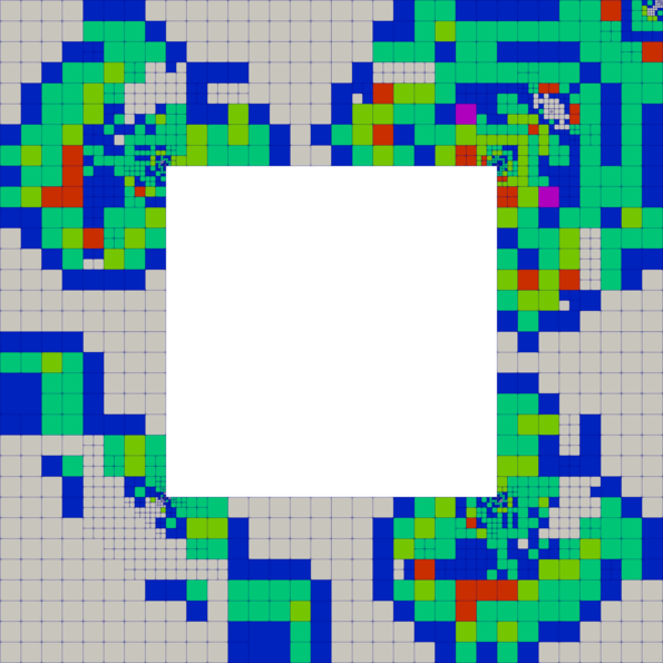
While this is certainly not a perfect arrangement, it does make some sense: we use low order elements close to boundaries and corners where regularity is low. On the other hand, higher order elements are used where (i) the error was at one point fairly large, i.e. mainly in the general area around the corner singularities and in the top right corner where the solution is large, and (ii) where the solution is smooth, i.e. far away from the boundary.
This arrangement of polynomial degrees of course follows from our smoothness estimator. Here is the estimated smoothness of the solution, with darker colors indicating least smoothness and lighter indicating the smoothest areas:
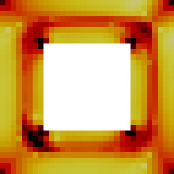
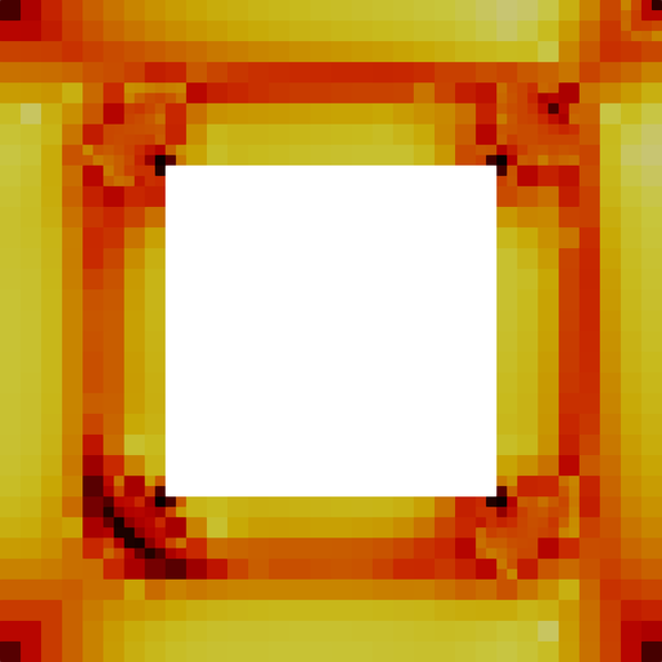
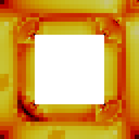
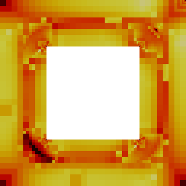
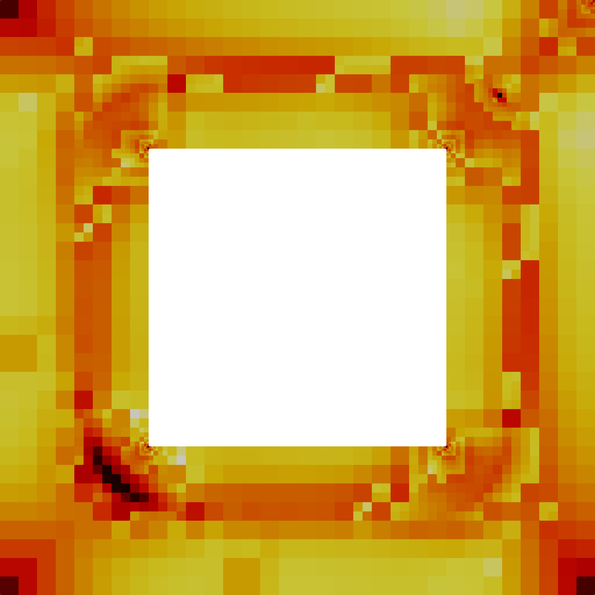

The primary conclusion one can draw from this is that the loss of regularity at the internal corners is a highly localized phenomenon; it only seems to impact the cells adjacent to the corner itself, so when we refine the mesh the black coloring is no longer visible. Besides the corners, this sequence of plots implies that the smoothness estimates are somewhat independent of the mesh refinement, particularly when we are far away from boundaries. It is also obvious that the smoothness estimates are independent of the actual size of the solution (see the picture of the solution above), as it should be. A point of larger concern, however, is that one realizes on closer inspection that the estimator we have overestimates the smoothness of the solution on cells with hanging nodes. This in turn leads to higher polynomial degrees in these areas, skewing the allocation of finite elements onto cells.
We have no good explanation for this effect at the moment. One theory is that the numerical solution on cells with hanging nodes is, of course, constrained and therefore not entirely free to explore the function space to get close to the exact solution. This lack of degrees of freedom may manifest itself by yielding numerical solutions on these cells with suppressed oscillation, meaning a higher degree of smoothness. The estimator picks this signal up and the estimated smoothness overestimates the actual value. However, a definite answer to what is going on currently eludes the authors of this program.
The bigger question is, of course, how to avoid this problem. Possibilities include estimating the smoothness not on single cells, but cell assemblies or patches surrounding each cell. It may also be possible to find simple correction factors for each cell depending on the number of constrained degrees of freedom it has. In either case, there are ample opportunities for further research on finding good \(hp\) refinement criteria. On the other hand, the main point of the current program was to demonstrate using the \(hp\) technology in deal.II, which is unaffected by our use of a possible sub-optimal refinement criterion.
 1.8.14