
deal.II version GIT relicensing-6842-g793a97d2aa 2026-10-02 14:00:01+00:00
\(\newcommand{\dealvcentcolon}{\mathrel{\mathop{:}}}\) \(\newcommand{\dealcoloneq}{\dealvcentcolon\mathrel{\mkern-1.2mu}=}\) \(\newcommand{\jump}[1]{\left[\!\left[ #1 \right]\!\right]}\) \(\newcommand{\average}[1]{\left\{\!\left\{ #1 \right\}\!\right\}}\)
Loading...
Searching...
No Matches
The step-100 tutorial program

This tutorial depends on step-7.

Table of contents
  1. Introduction
  2. The commented program
  1. Results
  2. The plain program

This program was contributed by Oreste Marquis (Polytechnique Montréal), Bruno Blais (Polytechnique Montréal), and Matthias Maier (Texas A&M). Bruno Blais acknowledges funding from the Natural Sciences and Engineering Research Council of Canada (NSERC) through Discovery Grant RGPIN-2020-04510, the Canada Research Chair (Level 2) in Computer-Assisted Design and Scale-Up of Alternative Energy Vectors for Sustainable Chemical Processes (CRC-2022-00340) under the Multiphysics Multiphase Intensification Automatization Workbench (MMIAOW), as well as computational resources provided by the Digital Alliance of Canada.

Introduction

As a follow up to the Helmholtz equation "with the nice sign" of step-7, here we will consider the version of the equation with the "bad sign", commonly referred to as the indefinite Helmholtz equation:

\[ -\Delta u - \alpha u = f. \]

This equation naturally arises in the study of time-harmonic wave phenomena, such as electromagnetic or acoustic propagation. In particular, it corresponds to the time-independent form of the wave equation when \(\alpha = \omega^2\) is the square of the angular frequency.

From a numerical perspective, solving this equation poses a number of well-known challenges, which become increasingly severe as the parameter \(\alpha > 0\) grows. Notably, the oscillatory nature of the solution requires the wavelength to be adequately resolved by the discretization and \(\alpha\) must not coincide with an eigenvalue of \(-\Delta\) or the resulting operator will not be invertible. Another difficulty that is really challenging is the indefiniteness of the operator. It hinders the ability of classical iterative methods (e.g. Krylov subspace methods) to solve the linear system of equations. Furthermore, most blackbox preconditioners fail to improve convergence as explained in detail by O. Ernst and M. J. Gander [89]. A solution to this problem is to make our discretized system of equations positive definite, which brings us to the subject of this tutorial: the Discontinuous Petrov-Galerkin (DPG) method [79]. This approach can be classified as a residual minimization method and always yields an Hermitian positive definite stiffness matrix system. It follows that using this method allows for the use of the preconditioned conjugate gradient (CG) linear solver instead of a direct solver or a more complex iterative method such as GMRES. This alone has the desired effect of reducing the memory consumption of the simulation, which enables the simulation of larger problems (i.e., higher frequencies or larger domains).

The numerical implementation of DPG shares many similarities with hybridizable discontinuous Galerkin (HDG) methods. In particular, it relies on trace elements to couple neighboring cells and on discontinuous Galerkin elements for the interior unknowns. In addition, the resulting linear system has an analogous structure that allows static condensation to reduce the system size by eliminating interior unknowns through a Schur-complement procedure. For readers who want to learn more about the implementation of trace unknowns, static condensation, and HDG formulations, step-51 provides a detailed introduction.

The time-harmonic Helmholtz equation

For our case study of the indefinite Helmholtz equation, we consider the linear acoustic equations in a 2D square domain \([0,1] \times [0,1]\). These equations arise from the linearization of the compressible inviscid fluid dynamics description (Euler equations) about a quiescent background state (no flow) and read:

\begin{align*} \frac{\partial \mathbf{U}}{\partial t} & = - \frac{1}{\rho }\nabla P \quad \text{in } \Omega, \qquad \text{(Linear momentum),}\\ \frac{1}{\kappa}\frac{\partial P}{\partial t} & = - \nabla \cdot \mathbf{U}, \quad \text{in } \Omega \qquad \text{(Mass conservation)}. \end{align*}

Here, \(\mathbf{U}(\mathbf{x},t)\) denotes the velocity perturbation, \(P(\mathbf{x},t)\) the pressure perturbation, \(\rho\) the mean fluid density, and \(\kappa\) its bulk modulus. Assuming that both pressure and velocity perturbations are time-harmonic with angular frequency \(\omega\), i.e.,

\begin{align*} \mathbf{U}(\mathbf{x},t)= \mathbf{u}(\mathbf{x})e^{i\omega t}, \qquad P(\mathbf{x},t)= p(\mathbf{x})e^{i\omega t}, \end{align*}

we can substitute this ansatz into the time-dependent equations to evaluate the time derivative. Then, by dividing out the common factor \(e^{i\omega t}\), we recover the frequency-domain system of equations:

\begin{align*} i\omega \mathbf{u} + \nabla p^* & = 0, \quad \text{in } \Omega,\\ i \frac{\omega}{c_s^2} p^* + \nabla \cdot \mathbf{u} & = 0, \quad \text{in } \Omega. \end{align*}

In the above, we have introduced the kinematic pressure \(p^* = p/\rho\) and the speed of sound \(c_s = \sqrt{\kappa/\rho}\) for notational convenience. At first glance, this first-order system does not resemble the indefinite Helmholtz equation for the acoustic pressure. However, by isolating \(\mathbf{u}\) from the linear momentum equation, substituting it into the mass conservation equation, and multiplying the resulting expression by \(i\omega\), we recover the classical second-order form:

\begin{align*} -\Delta p^* - \frac{\omega^2}{c_s^2}p^* & = 0, \end{align*}

This corresponds to the homogeneous Helmholtz equation with \(\alpha = \omega^2 / c_s^2\), and the special case \(f = 0\) of the general indefinite Helmholtz problem. In what follows, we will keep \(f=0\), but the source term \(f\) could be reintroduced, if desired, in the mass conservation equation. This would simply imply that there is mass injection or extraction in the domain. Another simplification that we will make in this tutorial is to consider \(c_s=1\).

Nonetheless, we will define our problem in such a way that we can implement and describe all the possible types of boundary conditions on \(\Gamma\) to showcase their different definitions in a DPG framework. Those are defined as:

\begin{align*} p^* & = g_D, \quad \text{on } \Gamma_0, \\ \mathbf{u} \cdot \mathbf{n} & = g_N, \quad \text{on } \Gamma_2, \\ \mathbf{u} \cdot \mathbf{n} - \frac{ k_n }{\omega} p^* & = g_R, \quad \text{on } \Gamma_1 \cup \Gamma_3, \end{align*}

where the subscript numbers follow the same nomenclature as the one for a rectangular geometry obtained from the GridGenerator::hyper_cube() function, \(k_n\) is the wavenumber in the direction of the surface normal and \(g_{D,N,R}\) refers to Dirichlet, Neumann and Robin boundary condition terms. To validate our implementation and showcase how DPG enables the computation of high frequency regime problems (i.e., \(\omega L / c_s \gg 1\) or in our case study \(\omega \gg 1\)), we choose the boundaries so the expected solution is a plane wave traveling in the direction \(\theta \in [0, \pi /2]\), i.e.:

\begin{align*} g_D &= e^{-i k y \sin(\theta)},\\ g_N &= -\sin(\theta) e^{-i k x \cos(\theta)},\\ g_R &= 0. \end{align*}

The expected analytical solution of our problem is therefore:

\begin{align*} p^* & = e^{-i k (x \cos(\theta) + y \sin(\theta))}, \\ \mathbf{u} & = \frac{1}{c_s} \begin{pmatrix} \cos(\theta) \\ \sin(\theta) \end{pmatrix} e^{-i k (x \cos(\theta) + y \sin(\theta))}. \end{align*}

Note that the wavenumber \(k\) introduced above for the plane-wave solution is chosen to satisfy \(k = \omega/c_s = \sqrt{\alpha}\). In this way, the scale of the oscillations in the solution is consistent with the natural wavelength of the Helmholtz operator.

To solve the acoustic linear system presented above using FEM, it is common to use the classical second-order form and multiply it by a test function \(q\) to obtain the following weak variational formulation:

\begin{align*} \text{Find } & p^* \in H^1(\Omega) \text{ so that}\\ & (\nabla q, \nabla p^*) - \omega^2 (q, p^*) - \langle q, \frac{\partial p^*}{\partial n} \rangle_{\Gamma} = 0, \quad \forall q \in H^1(\Omega). \end{align*}

Note that in this tutorial, we used everywhere the following definitions for the (sesquilinear) \(L^2\) complex inner products on the domain \(\Omega\) and its boundary \(\Gamma\):

\begin{align*} (a,b)_\Omega & := \int_{\Omega} \overline{a} b \text{d}x \approx \sum_{K\in \Omega_h} \int_{K} \overline{a} b \text{d}x & & \langle a,b \rangle_{\Gamma} := \int_{\Gamma} \overline{a}b \text{d}s \approx \sum_{\partial K \in\Gamma_h} \int_{\partial K} \overline{a}b \text{d}s, \end{align*}

where \(\Omega_h = \bigcup K\) is the discretized domain with elements \(K\), and \(\Gamma_h = \bigcup \partial K\) is the discretized boundary with \(dim-1\) elements \(\partial K\).

In the DPG literature, this weak formulation of the second-order equation is referred to as the primal formulation. While widely used, there are other ways to weaken the strong form of the problem. Notably, there is one that is referred to as the ultraweak formulation. This alternative representation is obtained by using the first-order system presented above and relaxing both equations independently. This is the form that we will use and solve in this tutorial since previous DPG studies have shown that the problem formulated in this manner leads to better results because of its approximability properties. To obtain it, we will use the vector-valued test function \(\mathbf{v}\) to weaken the mass conservation equation and the scalar test function \(q\) to weaken the linear momentum equation. The resulting ultraweak variational formulation of our indefinite Helmholtz problem is then:

\begin{align*} \text{Find } & p^* \in L^2(\Omega) \text{ and } \mathbf{u} \in (L^2(\Omega))^d \text{ so that} \\ & ( \mathbf{v}, i \omega \mathbf{u})_{\Omega_h} - (\nabla \cdot \mathbf{v}, p^*)_{\Omega_h} + \langle \mathbf{v} \cdot \mathbf{n}, p^* \rangle_{\Gamma} = 0, \quad \forall \mathbf{v} \in H(\text{div}, \Omega), \\ &(q, i\omega p^*)_{\Omega_h} - (\nabla q, \mathbf{u})_{\Omega_h} + \langle q, \mathbf{u} \cdot \mathbf{n} \rangle_{\Gamma} = 0, \quad \forall q \in H^1(\Omega). \end{align*}

The Discontinuous Petrov-Galerkin Method

There are numerous papers that describe the mathematics behind the DPG method, here we will focus mainly on the key elements necessary to understand the numerical implementation. Let’s start with a standard abstract problem defined on the product of the trial and test Hilbert spaces \(U \times V\) such that:

\begin{equation*} \begin{cases} b(v,u) = l(v) \quad \forall v \in V, \\ u \in U, \end{cases} \end{equation*}

where \(b(u,v)\) is a continuous bilinear form and \(l(v)\) is a continuous linear form. Furthermore, we assume that the problem is well-posed (i.e., \(b\) is coercive, or satisfies a continuous inf-sup condition). This can be reformulated as an operator equation by defining the operator \(B: U \rightarrow V'\) such that:

\begin{equation*} b(v,u) = \langle v, B u \rangle_{V \times V'}, \end{equation*}

where \(V'\) is the dual space of \(V\) and the \(\langle \cdot, \cdot \rangle_{V \times V'}\) denotes the duality pairing. This is one possible FEM discretization, typically referred to as the "Galerkin least squares method", where the residual in the dual norm is minimized over a finite-dimensional trial space. This finite element discretization leads to the following minimal residual formulation of the problem:

\begin{equation*} u_h = \arg \min_{w_h \in U_h} J(w_h), \quad \text{where} \quad J(w_h) = \frac{1}{2} \| l - B w_h \|_{V'}^2 \end{equation*}

where \(u_h\) is the discrete approximated solution. However, numerically computing the dual norm is not always feasible, so it is avoided by introducing a Riesz operator \(R: V \rightarrow V'\). Using the inverse Riesz operator, it is now possible to formulate an alternative discrete problem as:

\begin{equation*} u_h = \arg \min_{w_h \in U_h} \frac{1}{2} \| R^{-1}(l - B w_h) \|_{V}^2. \end{equation*}

This solves the problem of computing the norm of the dual space. Still, we now require the inverse Riesz operator. This is not achievable numerically because the Riesz map is related to the infinite-dimensional space \(V\) and its inversion is equivalent to solving a partial differential equation. To overcome this, the test space is "broken" between each individual element and enriched by raising its polynomial degree by \(\Delta p\) (typically chosen to be 1 or 2) compared to the trial space. The resulting finite-dimensional space \(V^r \subset V\) is now a truncated version of the original space, nonetheless, it can fully represent the Riesz map on each element by the Gram matrix. The broken test functions have no conformity assumptions across the inter-element boundaries, but they leave uncanceled interface terms, and thus require the introduction of interface unknowns (often called trace variables, or Lagrange multipliers \(\hat{u}\)) that live on the mesh skeleton and weakly enforce the continuity. With all those additional requirements, the final form of the abstract problem that needs to be solved in a DPG setting is:

\begin{equation*} \label{eq:DPG_abstract_problem} \begin{cases} \text{Find } u_h \in U_h \subset U, \quad \hat{u}_h \in \hat{U}_h \subset \hat{U} \text{ and } \quad \Psi^r \in V^r(\Omega_h) \text{ so that } \\ (v^r, \Psi^r )_V + b_h(v^r, u_h) + \langle v^r, \hat{u}_h \rangle = l(v^r), \quad \forall v^r \in V^r(\Omega_h), \\ b_h(w_h, \Psi^r) = 0, \quad \forall w_h \in U_h, \\ \langle \hat{w}_h, \Psi^r \rangle = 0, \quad \forall \hat{w}_h \in \hat{U}_h, \end{cases} \end{equation*}

where \(\Psi^r = R^{-1}_r(l-Bu_h)\). Finally, by defining the bases for discretized trial space \(U_h \times \hat{U}_h\) and the discretized broken test space \(V^r(\Omega_h)\), such that \(U_h = \text{span}\{ \phi_i \}_{i=1}^{N_u}\), \(\hat{U}_h = \text{span}\{ \hat{\phi}_i \}_{i=1}^{N_{\hat{u}}}\) and \(V^r= \text{span}\{ \Psi_i \}_{i=1}^{N_v}\), where \(N_v > N_u + N_{\hat{u}}\), the problem can be solved numerically by:

\begin{equation*} \text{Finding the set of coefficients } \mathbf{w} = [w_i]_{i=1}^{N_u} \in \mathbb{F}^{N_u}, \hat{\mathbf{w}} = [\hat{w}_i]_{\hat{i}=1}^{N_{\hat{u}}} \in \mathbb{F}^{N_{\hat{u}}}, \text{ and } \mathbf{t} = [t_i]_{i=1}^{N_v} \in \mathbb{F}^{N_v}, \text{ so that }\\ u_h = \sum_{i=1}^{N_u} w_i \phi_i, \quad \hat{u}_h = \sum_{i=1}^{N_{\hat{u}}} \hat{w}_i \hat{\phi}_i, \quad \Psi^r = \sum_{i=1}^{N_v} t_i \Psi_i \text{ satisfy } \\ \begin{pmatrix} G & B & \hat{B} \\ B^\textsf{H} & 0 & 0 \\ \hat{B}^\textsf{H} & 0 & 0 \end{pmatrix} \begin{pmatrix} \Psi^r \\ u_h \\ \hat{u}_h \end{pmatrix} = \begin{pmatrix} l \\ 0 \\ 0 \end{pmatrix}. \end{equation*}

Note that in the above matrix, we made use of the \(^\textsf{H}\) symbol to denote the conjugate transpose operation and the Number set symbol \(\mathbb{F} = \mathbb{R}\) or \(\mathbb{C}\) as a place holder for real or complex sets. Solving this system of linear equations is analogous to solving a general overdetermined system in a least squares sense with a residual \(\Psi^r\). This is why the DPG method always produces Hermitian positive definite systems of equations. Furthermore, it shows that \(\Psi^r\) can be used to obtain an error indicator for adaptive hp-refinement.

Polynomial spaces

As presented above, the DPG method is based on the idea that the test space is not bound to the same space as the one for the trial space and that it can be chosen to maximize the accuracy and the stability of the numerical method. Consequently, to implement the DPG method for any set of equations, one needs to be able to discretize the whole exact sequence of energy spaces, which in 3D takes the form:

\[ H^1 \xrightarrow{\nabla} H(\mathrm{curl}) \xrightarrow{\nabla \times} H(\mathrm{div}) \xrightarrow{\nabla \cdot} L^2 \]

These spaces are defined as:

\begin{align*} & H^1(\Omega) = \{ u : \Omega \to \mathbb{R}(\mathbb{C}) : u \in L^2(\Omega), \nabla u \in (L^2(\Omega))^3 \} \\ & H(\text{curl}, \Omega) = \{ \mathbf{E} : \Omega \to \mathbb{R}^3(\mathbb{C}^3) : \mathbf{E} \in (L^2(\Omega))^3, \nabla \times \mathbf{E} \in (L^2(\Omega))^3 \} \\ & H(\text{div}, \Omega) = \{ \mathbf{v} : \Omega \to \mathbb{R}^3(\mathbb{C}^3) : \mathbf{v} \in (L^2(\Omega))^3, \nabla \cdot \mathbf{v} \in L^2(\Omega) \} \\ & L^2(\Omega) = \{ q : \Omega \to \mathbb{R}(\mathbb{C}) : \|q\| < \infty \} \end{align*}

To obtain a finite-dimensional approximation, each of these infinite-dimensional spaces is discretized using polynomial basis functions of degree \(p\). The sequence of elements that can be used on the mesh \(\Omega_h\) then takes the form:

\[ Q_p \xrightarrow{\nabla} \mathbf{N}_p \xrightarrow{\nabla \times} \mathbf{RT}_p \xrightarrow{\nabla \cdot} DGQ_p \]

where \(p\) denotes the polynomial degree, \(Q_p\) the continuous Lagrange elements used to approximate \(H^1\), \(\mathbf{N}_p\) the Nédélec elements for \(H(\mathrm{curl})\), \(\mathbf{RT}_p\) the Raviart-Thomas elements for \(H(\mathrm{div})\), and \(DGQ_p\) the discontinuous Lagrange elements for \(L^2\).

In addition, the continuity requirements along faces and edges (the skeleton of the mesh), is also enforced with different spaces because these spaces live in \(dim -1\) dimensions. Thus, we also need to define the following spaces for the skeleton:

\begin{align*} H^{1/2}(\partial K) & = \text{tr}_{\text{grad}}(H^1(\Omega_h)) := \prod_{K \in \Omega_h} u\big|_{\partial K} \\ H^{-1/2}(\text{curl}, \partial K) & = \text{tr}_{\text{curl}, \top}(H(\text{curl}, \Omega_h)) := \prod_{K \in \Omega_h} (\mathbf{n}_K \times \mathbf{E}) \times \mathbf{n}_K \big|_{\partial K} \\ H^{-1/2}(\text{div}, \partial K) & = \text{tr}_{\text{curl}, \dashv }(H(\text{curl}, \Omega_h)) := \prod_{K \in \Omega_h} (\mathbf{n}_K \times \mathbf{E}) \big|_{\partial K} \\ H^{-1/2}(\partial K) & = \text{tr}_{\text{div}}(H(\text{div}, \Omega_h)) := \prod_{K \in \Omega_h} (\mathbf{n}_K \cdot \textbf{v} ) \big|_{\partial K} \end{align*}

Their discrete approximations are obtained by applying the corresponding trace operators to the associated volumetric discrete elements presented above.

Application to the acoustic Helmholtz equation

Now if we apply the DPG method to the acoustic Helmholtz ultraweak formulation presented above, we get the following:

\begin{align*} \text{Find } & p^* \in L^2(\Omega_h), \mathbf{u} \in (L^2(\Omega_h) )^d, \hat{p}^* \in H^{1/2}(\partial \Omega_h) \text{ and } \hat{u}_n \in H^{-1/2}(\partial \Omega_h) \text{ so that} \\ & ( \mathbf{v}, i \omega\mathbf{u})_{\Omega_h} - (\nabla \cdot \mathbf{v}, p^*)_{\Omega_h} + \langle \mathbf{v} \cdot \mathbf{n}, \hat{p}^* \rangle_{\partial \Omega_h} = 0, \quad \forall \mathbf{v} \in H(\text{div}, K), \\ &(q, i\omega p^*)_{\Omega_h} - (\nabla q, \mathbf{u})_{\Omega_h} + \langle q, \hat{u}_n \rangle_{\partial \Omega_h} = 0, \quad \forall q \in H^1(K). \end{align*}

where we make explicit the difference between the interior terms \(\mathbf{u}\) and \(p^*\) and the mesh interface terms \(\hat{u}_n\) and \(\hat{p}^*\), which live on the skeleton ( \(\partial \Omega_h\)). From this ultraweak formulation, we can identify the functional space of our problem:

\begin{align*} & U = (L^2(\Omega))^{dim} \times L^2(\Omega) \times H^{-1/2}(\partial \Omega_h) \times H^{1/2}(\partial \Omega_h) , \\ & V = H(\text{div}, K) \times H^1(K). \end{align*}

We can also directly define the adjoint graph norm which will be used to build the Gram matrix and control the residual:

\begin{equation*} \|(\mathbf{v}, q)\|^2_V := \|A^* (\mathbf{v}, q)\|^2 + \beta^2 (\|\mathbf{v}\|^2 + \|q\|^2 )= \|\ i\omega \mathbf{v} + \nabla q \|^2 + \| i\omega q + \nabla \cdot \mathbf{v}\|^2 + \|\mathbf{v}\|^2 + \|q\|^2, \end{equation*}

where \(\beta = \mathcal{O}(1)\) is a scaling parameter necessary for the stability of the method (here chosen to be one as it is commonly done in the literature).

Implementation of the boundary conditions

When using the ultraweak form, we can readily implement both Dirichlet and Neumann boundary conditions. The latter is in fact a Dirichlet boundary condition on the flux variable of our problem, here the fluid velocity. However, careful attention needs to be given to Robin boundary conditions because they tie together the two fields of interest and we do not want to overconstrain the system. To do so, here we will present the method proposed by J. Gopalakrishnan and J. Schöberl [110]. We therefore add an approximate version of the \(\mathbf{u} \cdot \mathbf{n} - \frac{ k_n }{\omega} p^* = g_R\) into our system by adding the term:

\begin{align*} \pm \bigg\langle \hat{w}_n - \frac{ k_n}{\omega} \hat{r}^*, \hat{u}_n - \frac{ k_n}{\omega} \hat{p}^* \bigg \rangle_{\Gamma_1 \cup \Gamma_3} = \pm \bigg\langle \hat{w}_n - \frac{ k_n}{\omega} \hat{r}^*, g_R \bigg \rangle_{\Gamma_1 \cup \Gamma_3}, \quad \forall \hat{w}_n \in H^{1/2}(\Gamma_1 \cup \Gamma_3), \hat{r}^* \in H^{-1/2}(\Gamma_1 \cup \Gamma_3) \end{align*}

on the appropriate boundaries. This extra relation adds new terms in the third equation of the DPG abstract formulation and changes the overall structure to the following:

\begin{equation*} \begin{pmatrix} G & B & \hat{B} \\ B^\textsf{H} & 0 & 0 \\ \hat{B}^\textsf{H} & 0 & D \end{pmatrix} \begin{pmatrix} \Psi^r \\ u_h \\ \hat{u}_h \end{pmatrix} = \begin{pmatrix} l \\ 0 \\ g_R \end{pmatrix}. \end{equation*}

In the above, we choose the sign so that the whole system remains positive definite (i.e., the matrix \(D\) needs to be negative semidefinite, so we choose the negative sign). As a final consequence of the Robin boundary condition, we also want to control the residual on this type of boundary. Therefore, we need to modify the adjoint graph norm to take the new terms into account as follows:

\begin{align*} \|(\mathbf{v}, q)\|^2_E = \|i\omega \mathbf{v} + \nabla q \|^2 + \|i\omega q + \nabla \cdot \mathbf{v}\|^2 + \|\mathbf{v}\|^2 + \|q\|^2 + \|\mathbf{v} \cdot \mathbf{n} + \frac{k_n}{\omega} q\|^2_{\Gamma_1 \cup \Gamma_3}. \end{align*}

We are now finally ready to build the following DPG system for our problem:

\begin{equation*} \begin{pmatrix} (\mathbf{v}, \mathbf{v})_{\Omega_h} + (\nabla \cdot \mathbf{v}, \nabla \cdot \mathbf{v})_{\Omega_h} + (i\omega\mathbf{v}, i\omega \mathbf{v})_{\Omega_h} + \langle \mathbf{v} \cdot \mathbf{n}, \mathbf{v} \cdot \mathbf{n} \rangle_{\Gamma_1 \cup \Gamma_3} & (i\omega \mathbf{v}, \nabla q)_{\Omega_h} + (\nabla \cdot \mathbf{v}, i\omega q)_{\Omega_h} + \langle \mathbf{v} \cdot \mathbf{n}, \frac{k_n}{\omega}q \rangle_{\Gamma_1 \cup \Gamma_3} & ( \mathbf{v}, i\omega \mathbf{u})_{\Omega_h} & -( \nabla \cdot \mathbf{v}, p^*)_{\Omega_h} & 0 & \langle \mathbf{v} \cdot \mathbf{n}, \hat{p}^* \rangle_{\partial \Omega_h} \\ (\nabla q, i\omega \mathbf{v})_{\Omega_h} + ( i\omega q, \nabla \cdot \mathbf{v})_{\Omega_h} + \langle \frac{k_n}{\omega}q, \mathbf{v} \cdot \mathbf{n} \rangle_{\Gamma_1 \cup \Gamma_3} & (q, q)_{\Omega_h} + (\nabla q, \nabla q)_{\Omega_h} + ( i\omega q, i\omega q)_{\Omega_h} + \langle \frac{k_n}{\omega}q, \frac{k_n}{\omega}q \rangle_{\Gamma_1 \cup \Gamma_3} & - (\nabla q,\mathbf{u})_{\Omega_h} & (q, i\omega p^*)_{\Omega_h}& \langle q, \hat{u}_n \rangle_{\partial \Omega_h} & 0 \\ (i\omega \mathbf{u}, \mathbf{v})_{\Omega_h} & -(\mathbf{u}, \nabla q )_{\Omega_h} & 0 & 0 & 0 & 0 \\ -(p^*, \nabla \cdot \mathbf{v} )_{\Omega_h} & ( i\omega p^*, q)_{\Omega_h} & 0 & 0 & 0 & 0 \\ 0 & \langle \hat{u}_n, q \rangle_{\partial \Omega_h} & 0 & 0 & - \langle \hat{u}_n, \hat{u}_n \rangle_{\Gamma_1 \cup \Gamma_3} & \langle \hat{u}_n, \frac{k_n}{\omega} \hat{p}^* \rangle_{\Gamma_1 \cup \Gamma_3} \\ \langle \hat{p}^*, \mathbf{v} \cdot \mathbf{n} \rangle_{\partial \Omega_h} & 0 & 0 & 0 & \langle \frac{k_n}{\omega} \hat{p}^*, \hat{u}_n \rangle_{\Gamma_1 \cup \Gamma_3} & - \langle \frac{k_n}{\omega} \hat{p}^*, \frac{k_n}{\omega} \hat{p}^* \rangle_{\Gamma_1 \cup \Gamma_3} \end{pmatrix} \begin{pmatrix} \mathbf{v} \\ q \\ \mathbf{u} \\ p^* \\ \hat{u}_n \\ \hat{p}^* \end{pmatrix} = \begin{pmatrix} (\mathbf{v}, l)_{\Omega_h} \\ (q,l)_{\Omega_h} \\ 0 \\ 0 \\ - \langle \hat{u}_n, g_R \rangle_{\Gamma_1 \cup \Gamma_3} \\ \langle \frac{k_n}{\omega} \hat{p}^*, g_R \rangle_{\Gamma_1 \cup \Gamma_3} \end{pmatrix} \end{equation*}

where we left the terms \(l\) and \(g_R\) in the formulation even if those are null in our case study for clarity.

Final elementary system and condensation

Finally, because the Gram matrix is block-diagonal, where each block corresponds to a cell, it is common to condense it in order to remove the residual unknowns. The resulting system is:

\begin{equation*} \begin{pmatrix} B^\textsf{H} G^{-1}B & B^\textsf{H} G^{-1}\hat{B} \\ \hat{B}^\textsf{H} G^{-1}B & \hat{B}^\textsf{H} G^{-1}\hat{B} - D \end{pmatrix} \begin{pmatrix} u_h \\ \hat{u}_h \end{pmatrix} = \begin{pmatrix} B^\textsf{H} G^{-1}l \\ \hat{B}^\textsf{H} G^{-1}l - g \end{pmatrix}, \end{equation*}

where \(u_h = \{\mathbf{u},p^*\}\) and \(\hat{u}_h = \{\hat{u}_n,\hat{p}^*\}\). To avoid extra computational cost when solving the system, it can be further condensed to solve only for the interface degrees of freedom since the interior degrees of freedom are discontinuous across elements and can be locally condensed. By posing the following:

\begin{align*} & M_1 = B^\textsf{H} G^{-1}B, & M_2 = B^\textsf{H} G^{-1}\hat{B}, && M_3 = \hat{B}^\textsf{H} G^{-1}\hat{B} - D, && M_4 = B^\textsf{H} G^{-1} && M_5 = \hat{B}^\textsf{H} G^{-1}, \end{align*}

we can simply solve the system:

\begin{equation*} (M_3 - M_2^\textsf{H} M_1^{-1} M_2) \hat{u}_h = (M_5 - M_2^\textsf{H} M_1^{-1} M_4) l - g, \end{equation*}

to obtain the solution on the faces of the mesh and then use it to recover the solution \(u_h\) in the interiors of cells, with the following relation:

\begin{equation*} u_h = M_1^{-1} (M_4 l - M_2 \hat{u}_h). \end{equation*}

This is the method that is presented in the code that follows.

The commented program

Include files

The DPG method requires a large breadth of element types which are included below. Beside these, the rest of the includes are some well-known files used in many other tutorials. We also define the constant pi for later use across the file and we encapsulate everything in the Step100 namespace.

  #include <deal.II/fe/fe_dgq.h>
  #include <deal.II/fe/fe_face.h>
  #include <deal.II/fe/fe_q.h>
  #include <deal.II/fe/fe_raviart_thomas.h>
  #include <deal.II/fe/fe_trace.h>
  #include <deal.II/base/convergence_table.h>
  #include <deal.II/base/function.h>
  #include <deal.II/base/quadrature_lib.h>
  #include <deal.II/base/tensor_function.h>
  #include <deal.II/dofs/dof_handler.h>
  #include <deal.II/dofs/dof_tools.h>
  #include <deal.II/fe/fe_system.h>
  #include <deal.II/fe/fe_values.h>
  #include <deal.II/grid/grid_generator.h>
  #include <deal.II/grid/grid_tools.h>
  #include <deal.II/grid/tria.h>
  #include <deal.II/lac/affine_constraints.h>
  #include <deal.II/lac/dynamic_sparsity_pattern.h>
  #include <deal.II/lac/lapack_full_matrix.h>
  #include <deal.II/lac/precondition.h>
  #include <deal.II/lac/solver_cg.h>
  #include <deal.II/lac/sparse_matrix.h>
  #include <deal.II/lac/vector.h>
  #include <deal.II/numerics/data_out.h>
  #include <deal.II/numerics/data_out_faces.h>
  #include <deal.II/numerics/vector_tools.h>
  #include <fstream>
  #include <iostream>
  const double pi = ::numbers::PI;
  namespace Step100
  {
  using namespace dealii;
*  *  *  struct InterferenceTaperTransform *  
constexpr double PI
Definition numbers.h:240

We first create the analytical solutions of the velocity field ( \(\mathbf{u}\)) and the pressure field ( \(p^*\)) in the following Function classes declaration. However, in this tutorial, we will avoid the use of deal.II's complex arithmetic capabilities and only use the complex functions that are defined in the C++ standard library. Consequently, in what follows, we will separate the real and imaginary components of our spaces. Therefore, we will also define two implementations of each function, one for the real component and one for the imaginary one.

We start by creating the analytical solution class for the kinematic pressure ( \(p^*\)). The analytical solution depends on the wavenumber \(k\) and the angle \(\theta\) which are passed to the constructor. Since we are splitting the solution into real and imaginary parts, we can directly take \(\Re(p^*) = \Re(e^{-i k (x \cos(\theta) + y \sin(\theta))}) = \cos(k (x \cos(\theta) + y \sin(\theta)))\) and \(\Im(p^*) = \Im(e^{-i k (x \cos(\theta) + y \sin(\theta))}) = -\sin(k (x \cos(\theta) + y \sin(\theta)))\). The same goes for the real and imaginary parts of the velocity field. The only difference is that the velocity field is a vector field, so it will be derived from the TensorFunction class and return a Tensor<1,dim> in the value function.

  template <int dim>
  class AnalyticalSolutionPressureReal : public Function<dim>
  {
  public:
  AnalyticalSolutionPressureReal(const double wavenumber, const double theta)
  : Function<dim>()
  , wavenumber(wavenumber)
  , theta(theta)
  {}
  virtual double value(const Point<dim> &p,
  const unsigned int component) const override;
  private:
  const double wavenumber;
  const double theta;
  };
  template <int dim>
  double AnalyticalSolutionPressureReal<dim>::value(
  const Point<dim> &p,
  const unsigned int /*component*/) const
  {
  return std::cos(wavenumber *
  (p[0] * std::cos(theta) + p[1] * std::sin(theta)));
  }
  template <int dim>
  class AnalyticalSolutionPressureImag : public Function<dim>
  {
  public:
  AnalyticalSolutionPressureImag(const double wavenumber, const double theta)
  : Function<dim>()
  , wavenumber(wavenumber)
  {}
  virtual double value(const Point<dim> &p,
  const unsigned int component) const override;
  private:
  const double wavenumber;
  const double theta;
  };
  template <int dim>
  double AnalyticalSolutionPressureImag<dim>::value(
  const Point<dim> &p,
  const unsigned int /*component*/) const
  {
  return -std::sin(wavenumber *
  (p[0] * std::cos(theta) + p[1] * std::sin(theta)));
  }
  template <int dim>
  class AnalyticalSolutionVelocityReal : public TensorFunction<1, dim>
  {
  public:
  AnalyticalSolutionVelocityReal(const double wavenumber, const double theta)
  : TensorFunction<1, dim>()
  , wavenumber(wavenumber)
  {}
  virtual Tensor<1, dim> value(const Point<dim> &p) const override;
  private:
  const double wavenumber;
  const double theta;
  };
  template <int dim>
  AnalyticalSolutionVelocityReal<dim>::value(const Point<dim> &p) const
  {
  Tensor<1, dim> return_value;
  return_value[0] =
  std::cos(theta) *
  std::cos(wavenumber * (p[0] * std::cos(theta) + p[1] * std::sin(theta)));
  return_value[1] =
  std::sin(theta) *
  std::cos(wavenumber * (p[0] * std::cos(theta) + p[1] * std::sin(theta)));
  return return_value;
  }
  template <int dim>
  class AnalyticalSolutionVelocityImag : public TensorFunction<1, dim>
  {
  public:
  AnalyticalSolutionVelocityImag(const double wavenumber, const double theta)
  : TensorFunction<1, dim>()
  , wavenumber(wavenumber)
  {}
  virtual Tensor<1, dim> value(const Point<dim> &p) const override;
  private:
  const double wavenumber;
  const double theta;
  };
  template <int dim>
  AnalyticalSolutionVelocityImag<dim>::value(const Point<dim> &p) const
  {
  Tensor<1, dim> return_value;
  return_value[0] =
  std::cos(theta) *
  -std::sin(wavenumber * (p[0] * std::cos(theta) + p[1] * std::sin(theta)));
  return_value[1] =
  std::sin(theta) *
  -std::sin(wavenumber * (p[0] * std::cos(theta) + p[1] * std::sin(theta)));
  return return_value;
  }
Definition point.h:111
#define AssertDimension(dim1, dim2)
*  *  *  ScaleZFunction< dim, Number, components >::ScaleZFunction *  component(component)
*  *  *  *  std::vector< Number > ThermoPlasticMaterial< dim, ViscoplasticYieldLaw, Number >::get_state_parameters   const
::VectorizedArray< Number, width > cos(const ::VectorizedArray< Number, width > &)
::VectorizedArray< Number, width > sin(const ::VectorizedArray< Number, width > &)

A similar class is required for the boundary values functions that will be applied to constrain the dofs. The main difference with the above function declaration is that the number of components will now be 4 because this function will be applied to our space of skeleton unknowns via VectorTools::interpolate_boundary_values. This space has 4 components, because the skeleton unknowns on faces for the velocity field are scalars from the definition \(\hat{u}_{n} = \mathbf{u} \cdot n\) and there are the real and imaginary parts of both fields. The returned value will be based on the following component convention:

  • component == 0 : real part of velocity skeleton;
  • component == 1 : imaginary part of velocity skeleton;
  • component == 2 : real part of pressure skeleton;
  • component == 3 : imaginary part of pressure skeleton.
  template <int dim>
  class BoundaryValues : public Function<dim>
  {
  public:
  BoundaryValues(const double wavenumber, const double theta)
  : Function<dim>(4)
  , wavenumber(wavenumber)
  , theta(theta)
  {}
  virtual double value(const Point<dim> &p,
  const unsigned int component) const override;
  private:
  double wavenumber;
  double theta;
  };
  template <int dim>
  double BoundaryValues<dim>::value(const Point<dim> &p,
  const unsigned int component) const
  {
  if (component == 0)
  {
  return -1 * (std::sin(theta) *
  std::cos(wavenumber * p[0] * std::cos(theta)));
  }
  else if (component == 1)
  {
  return std::sin(theta) * std::sin(wavenumber * p[0] * std::cos(theta));
  }
  else if (component == 2)
  {
  return std::cos(wavenumber * p[1] * std::sin(theta));
  }
  else if (component == 3)
  {
  return -std::sin(wavenumber * p[1] * std::sin(theta));
  }
  else
  {
  AssertThrow(false, ExcMessage("Invalid component for BoundaryValues"));
  return 0.0;
  }
  }
#define AssertThrow(cond, exc)

The DPGHelmholtz class declaration

Next let's declare the main class of this program. The main difference from other examples lies in the fact that we rely on multiple DoFHandler and FESystem objects. The DoFHandler objects that we rely on are the following:

  • The dof_handler_trial_interior is for the unknowns in the interior of the cells;
  • The dof_handler_trial_skeleton is for the unknowns in the skeleton;
  • The dof_handler_test is for the test functions. Although we do not use the unknowns associated with this DoFHandler, it enables us to evaluate the test functions we will use in DPG.

The same applies for the three FESystem objects: fe_system_trial_interior, fe_system_trial_skeleton and fe_system_test. In each one of these objects, we will store the relevant finite element space in the same order as for the BoundaryValues function. The first component will therefore always be related to the real part of the velocity, the second component to its imaginary part, the third component to the real part of the pressure and the fourth component to its imaginary part.

The constructor of the class takes four arguments that define the problem. The first two are related to the finite element spaces degree, i.e., degree defines the polynomial degree of the trial space and delta_degree defines the difference in degree between the trial and the test space. Since the test space needs to be enriched compared to the trial space in DPG, delta_degree must be at least 1 to ensure that the method is well posed. The last two arguments are related to the plane wave parameters. The parameter wavenumber defines the wavenumber \(k\) of the plane wave problem while theta defines the incident angle. That angle must be in the closed interval \([0, \pi/2]\) for the boundary conditions to make sense. All those restrictions are asserted in the constructor.

The class also provides a number of member functions that are responsible for setting up, solving, and postprocessing the DPG formulation. The setup_system() function initializes the three DoFHandler objects, the sparsity pattern, the system matrix, and the right-hand side vector. It also imposes both Dirichlet and Neumann boundary conditions using AffineConstraints. The function assemble_system(bool solve_interior) handles the assembly of the DPG system. It takes a boolean argument as input to indicate whether the assembly is being performed for the skeleton solve or for the interior reconstruction. When solve_interior = false, the bilinear and linear forms are assembled and the system is locally condensed so that the resulting global system only involves the skeleton unknowns. When solve_interior = true, the system is assembled again and the previously computed skeleton solution is used to reconstruct the interior solution variables. As mentioned in the introduction, this two-step approach is interesting to reduce the size of the global system that needs to be solved which helps for memory consumption and for the iterative solver convergence, but this requires assembling the system twice. The boolean flag introduced is interesting since it allows reusing the same assembly function for both steps and avoid code duplication. The last functions of the class are pretty standard and include solve_linear_system_skeleton(), that solves the resulting linear system, refine_grid(), which applies uniform refinement to the triangulation, output_results(), that writes both the skeleton and interior solutions to separate VTU files for visualization, and finally calculate_L2_error(), which computes the \(L^2\) norm of the error using the known analytical solution.

In addition to these member functions, the class defines a number of member variables that are used throughout the implementation. These include the triangulation, finite element systems, DoFHandler objects, solution vectors, linear system data structures, and a ConvergenceTable used to store the \(L^2\) error and related quantities. The coefficients defining the incident plane wave, namely the wavenumber and the angle of incidence, are also stored as class members. The class defines also several FEValuesExtractors variables that are reused at multiple points in the implementation to select the appropriate components of the finite element spaces for both the trial and test functions. These extractors provide access to the real and imaginary parts of the velocity and pressure variables. Since the skeleton space does not have the same number of components as the interior or test spaces (because the \(H^{-1/2}\) space associated with the velocity field is scalar) additional extractors are defined specifically for the skeleton variables.

  template <int dim>
  class DPGHelmholtz
  {
  public:
  DPGHelmholtz(const unsigned int degree,
  const unsigned int delta_degree,
  const double wavenumber,
  const double theta);
  void run();
  private:
  void setup_system();
  void assemble_system(bool solve_interior);
  void solve_linear_system_skeleton();
  void refine_grid(unsigned int cycle);
  void output_results(unsigned int cycle);
  void calculate_L2_error();
  Triangulation<dim> triangulation;
  const FESystem<dim> fe_trial_interior;
  DoFHandler<dim> dof_handler_trial_interior;
  Vector<double> solution_interior;
  const FESystem<dim> fe_trial_skeleton;
  DoFHandler<dim> dof_handler_trial_skeleton;
  Vector<double> solution_skeleton;
  Vector<double> system_rhs;
  SparsityPattern sparsity_pattern;
  SparseMatrix<double> system_matrix;
  const FESystem<dim> fe_test;
  DoFHandler<dim> dof_handler_test;
  ConvergenceTable error_table;
  const double wavenumber;
  const double theta;
  const FEValuesExtractors::Vector extractor_u_real;
  const FEValuesExtractors::Vector extractor_u_imag;
  const FEValuesExtractors::Scalar extractor_p_real;
  const FEValuesExtractors::Scalar extractor_p_imag;
  const FEValuesExtractors::Scalar extractor_u_hat_real;
  const FEValuesExtractors::Scalar extractor_u_hat_imag;
  const FEValuesExtractors::Scalar extractor_p_hat_real;
  const FEValuesExtractors::Scalar extractor_p_hat_imag;
  };

DPGHelmholtz Constructor

In the constructor, we assign the relevant finite element to each FESystem following the nomenclature described above:

  • fe_system_trial_interior contains \(\Re(\mathbf{u})\), \(\Im(\mathbf{u})\), \(\Re(p^*)\), \(\Im(p^*)\) ;
  • fe_system_trial_skeleton contains \(\Re(\hat{u}_n)\), \(\Im(\hat{u}_n)\), \(\Re(\hat{p}^*)\), \(\Im(\hat{p}^*)\) ;
  • fe_system_test contains \(\Re(\mathbf{v})\), \(\Im(\mathbf{v})\), \(\Re(q)\), \(\Im(q)\).

Note that the FE_Q and FE_TraceQ elements have a higher degree than the others because their numbering starts at 1 instead of 0. This is to ensure that the spaces chosen follow the exact sequence of energy spaces \(\text{Q}_{k+1} \rightarrow \text{Nédélec}_k \rightarrow \text{Raviart-Thomas}_k \rightarrow \text{DGQ}_k\). We also initialize the FEValuesExtractors that will be used according to our FESystems nomenclature. The constructor also includes assertions to check that the provided template parameter dim is equal to 2. The dimension is 2 because the problem is not implemented in 3D. We also verify that the delta_degree variable is at least 1 since the degree of the test space must be at least one degree higher than the trial space. Finally, we check that the wavenumber is positive since it is the magnitude of the wave vector and that the angle theta is in the interval \([0, \pi/2]\) because, as stated above, other angles would not be compatible with the current boundary definitions.

  template <int dim>
  DPGHelmholtz<dim>::DPGHelmholtz(const unsigned int degree,
  const unsigned int delta_degree,
  double wavenumber,
  double theta)
  : fe_trial_interior(FE_DGQ<dim>(degree) ^ dim,
  FE_DGQ<dim>(degree) ^ dim,
  FE_DGQ<dim>(degree),
  FE_DGQ<dim>(degree))
  , dof_handler_trial_interior(triangulation)
  , fe_trial_skeleton(FE_FaceQ<dim>(degree),
  FE_FaceQ<dim>(degree),
  FE_TraceQ<dim>(degree + 1),
  FE_TraceQ<dim>(degree + 1))
  , dof_handler_trial_skeleton(triangulation)
  , fe_test(FE_RaviartThomas<dim>(degree + delta_degree),
  FE_RaviartThomas<dim>(degree + delta_degree),
  FE_Q<dim>(degree + delta_degree + 1),
  FE_Q<dim>(degree + delta_degree + 1))
  , dof_handler_test(triangulation)
  , wavenumber(wavenumber)
  , theta(theta)
  , extractor_u_real(0)
  , extractor_u_imag(dim)
  , extractor_p_real(2 * dim)
  , extractor_p_imag(2 * dim + 1)
  , extractor_u_hat_real(0)
  , extractor_u_hat_imag(1)
  , extractor_p_hat_real(2)
  , extractor_p_hat_imag(3)
  {
  static_assert(dim == 2, "This tutorial example only works for dim==2");
  AssertThrow(delta_degree >= 1,
  ExcMessage("The delta_degree needs to be at least 1."));
  AssertThrow(wavenumber > 0, ExcMessage("The wavenumber must be positive."));
  AssertThrow(theta >= 0 && theta <= pi / 2,
  ExcMessage(
  "The angle theta must be in the interval [0, pi/2]."));
  }
Definition fe_q.h:552

DPGHelmholtz::setup_system

This function sets up the multiple DOFHandler objects and records the number of DoFs associated with each space in the ConvergenceTable for later reference. It also defines the constraints, but since the global linear system is posed exclusively in terms of the skeleton unknowns, constraints are only built for this corresponding DoFHandler. These include hanging-node constraints as well as boundary conditions. In particular, Dirichlet and Neumann boundary conditions are enforced on selected components of the skeleton variables by interpolating analytical boundary data onto the appropriate trace spaces using component masks and FEValuesExtractors. A Dirichlet condition is first applied to the pressure trace on the left boundary (types::boundary_id(0)), while a Neumann condition on the pressure is enforced by prescribing the normal component of the velocity trace on the bottom boundary (types::boundary_id(2)). Note that the Robin boundary conditions are not enforced through constraints and are instead incorporated later during the assembly of the bilinear and linear forms.

Once all constraints have been specified and closed, the vectors and matrices associated with the global linear system are initialized. Because the system only involves skeleton degrees of freedom, the sparsity pattern, system matrix, and right-hand side are constructed accordingly. The solution vectors for both the skeleton and interior unknowns are also initialized at this stage, preparing the class for the subsequent assembly and solution steps.

  template <int dim>
  void DPGHelmholtz<dim>::setup_system()
  {
  dof_handler_trial_skeleton.distribute_dofs(fe_trial_skeleton);
  dof_handler_trial_interior.distribute_dofs(fe_trial_interior);
  dof_handler_test.distribute_dofs(fe_test);
  std::cout << std::endl
  << "Number of dofs for the interior: "
  << dof_handler_trial_interior.n_dofs() << std::endl;
  error_table.add_value("dofs_interior", dof_handler_trial_interior.n_dofs());
  std::cout << "Number of dofs for the skeleton: "
  << dof_handler_trial_skeleton.n_dofs() << std::endl;
  error_table.add_value("dofs_skeleton", dof_handler_trial_skeleton.n_dofs());
  std::cout << "Number of dofs for the test space: "
  << dof_handler_test.n_dofs() << std::endl;
  error_table.add_value("dofs_test", dof_handler_test.n_dofs());
  constraints.clear();
  DoFTools::make_hanging_node_constraints(dof_handler_trial_skeleton,
  constraints);
  const BoundaryValues<dim> boundary_values(wavenumber, theta);
  VectorTools::interpolate_boundary_values(dof_handler_trial_skeleton,
  boundary_values,
  constraints,
  fe_trial_skeleton.component_mask(
  extractor_p_hat_real));
  VectorTools::interpolate_boundary_values(dof_handler_trial_skeleton,
  boundary_values,
  constraints,
  fe_trial_skeleton.component_mask(
  extractor_p_hat_imag));
  VectorTools::interpolate_boundary_values(dof_handler_trial_skeleton,
  boundary_values,
  constraints,
  fe_trial_skeleton.component_mask(
  extractor_u_hat_real));
  VectorTools::interpolate_boundary_values(dof_handler_trial_skeleton,
  boundary_values,
  constraints,
  fe_trial_skeleton.component_mask(
  extractor_u_hat_imag));
  constraints.close();
  solution_skeleton.reinit(dof_handler_trial_skeleton.n_dofs());
  system_rhs.reinit(dof_handler_trial_skeleton.n_dofs());
  solution_interior.reinit(dof_handler_trial_interior.n_dofs());
  DynamicSparsityPattern dsp(dof_handler_trial_skeleton.n_dofs());
  DoFTools::make_sparsity_pattern(dof_handler_trial_skeleton,
  dsp,
  constraints,
  false);
  sparsity_pattern.copy_from(dsp);
  system_matrix.reinit(sparsity_pattern);
  }
void make_hanging_node_constraints(const DoFHandler< dim, spacedim > &dof_handler, AffineConstraints< number > &constraints)
void make_sparsity_pattern(const DoFHandler< dim, spacedim > &dof_handler, SparsityPatternBase &sparsity_pattern, const AffineConstraints< number > &constraints={}, const bool keep_constrained_dofs=true, const types::subdomain_id subdomain_id=numbers::invalid_subdomain_id)
void interpolate_boundary_values(const Mapping< dim, spacedim > &mapping, const DoFHandler< dim, spacedim > &dof, const std::map< types::boundary_id, const Function< spacedim, number > * > &function_map, std::map< types::global_dof_index, number > &boundary_values, const ComponentMask &component_mask={})

DPGHelmholtz::assemble_system

This function incorporates the core difference of a DPG solver by assembling the local contributions of the bilinear and linear forms. In it, we begin by defining volume and face quadrature rules. Since the test space has a higher polynomial degree than the trial spaces by construction, the quadrature order is chosen based on the test finite element to ensure sufficient accuracy for all integrals. The number of quadrature points for both cell and face integration is also stored for later use.

Next, we create FEValues and FEFaceValues objects for the interior trial, skeleton trial, and test spaces. In the ultraweak formulation used here, gradients are only required for the test functions, while values are needed for all spaces. Because all spaces are defined on the same triangulation, the update of quadrature points and the transformation jacobian values is only required for one of the FEValues objects, which we choose to be the interior trial space.

We then query and store the number of degrees of freedom per cell associated with each finite element space. These values determine the sizes of all local matrices and vectors used during assembly. Notably, they are used to build containers to store shape function values, gradients, divergences, and their complex conjugates at each quadrature point to avoid repeated queries to FEValues objects. The first group of containers defined below corresponds to the test space quantities, including vector-valued test functions, their divergence, scalar test functions, and their gradients, both in the cell interior and on faces. The second group stores the interior trial variables, namely the velocity and pressure fields. The third group contains the skeleton trial variables, which represent the normal velocity and pressure traces and their complex conjugates.

Also with the goal of avoiding repeated queries when determining to which element a shape function belongs, we define an enum ShapeFunctionType that classifies shape functions into four categories: velocity real part, velocity imaginary part, pressure real part, and pressure imaginary part. It also defines two composite categories, one for all velocity shape functions and another for all pressure shape functions. This enumeration uses bits as boolean flags to facilitate efficient checks during assembly of the DPG matrices and vectors. Containers for these classifications are defined for each of the three finite element spaces with the size corresponding to the number of DoFs per cell in each space.

Then, the local DPG matrices are allocated. These include the Gram matrix \(G\) of the test space, the coupling matrix between test and interior trial spaces \(B\), the coupling matrix between test and skeleton trial spaces \(\hat{B}\), and the matrix \(D\) associated with skeleton coupling terms arising from Robin boundary conditions. In addition, local vectors corresponding to the linear functional in the test space \(l\) and to the skeleton trial space \(g\) are defined. Together, these matrices and vectors define the uncondensed local DPG system.

To perform the local static condensation, we need to allocate a set of auxiliary matrices that represent intermediate block operators arising in the elimination of interior degrees of freedom ( \(M_1\), \(M_2\), \(M_3\), \(M_4\) and \(M_5\) defined in the last section of the introduction). Further temporary matrices and vectors are also created to store intermediate results during matrix–matrix and matrix–vector products. These temporary objects are labeled with a "tmp" prefix.

Finally, we define the local cell matrix and right-hand side vector associated with the skeleton degrees of freedom that will be used to solve our system, together with a local-to-global DoF index map used for distribution into the global system. These are relevant to obtain the solution when solve_interior = false , but when solve_interior = true, we need to define additional vectors to store the interior solution, interior right-hand side, and the skeleton solution that will be used for the interior reconstruction step. Note that since the Helmholtz problem is complex-valued, we also define the imaginary unit and several complex constants that appear in the bilinear and linear forms. Although the global linear system that is built is real-valued, complex arithmetic from the C++ standard library is used locally to simplify the formulation, in the same spirit as in step-81.

  template <int dim>
  void DPGHelmholtz<dim>::assemble_system(const bool solve_interior)
  {
  const QGauss<dim> quadrature_formula(fe_test.degree + 1);
  const QGauss<dim - 1> face_quadrature_formula(fe_test.degree + 1);
  const unsigned int n_q_points = quadrature_formula.size();
  const unsigned int n_face_q_points = face_quadrature_formula.size();
  FEValues<dim> fe_values_trial_interior(fe_trial_interior,
  quadrature_formula,
  FEValues<dim> fe_values_test(fe_test,
  quadrature_formula,
  FEFaceValues<dim> fe_values_trial_skeleton(fe_trial_skeleton,
  face_quadrature_formula,
  FEFaceValues<dim> fe_face_values_test(fe_test,
  face_quadrature_formula,
  const unsigned int dofs_per_cell_test = fe_test.n_dofs_per_cell();
  const unsigned int dofs_per_cell_trial_interior =
  fe_trial_interior.n_dofs_per_cell();
  const unsigned int dofs_per_cell_trial_skeleton =
  fe_trial_skeleton.n_dofs_per_cell();
  std::vector<Tensor<1, dim, std::complex<double>>> v(dofs_per_cell_test);
  std::vector<Tensor<1, dim, std::complex<double>>> v_conj(
  dofs_per_cell_test);
  std::vector<std::complex<double>> div_v(dofs_per_cell_test);
  std::vector<std::complex<double>> div_v_conj(dofs_per_cell_test);
  std::vector<std::complex<double>> q(dofs_per_cell_test);
  std::vector<std::complex<double>> q_conj(dofs_per_cell_test);
  std::vector<Tensor<1, dim, std::complex<double>>> grad_q(
  dofs_per_cell_test);
  std::vector<Tensor<1, dim, std::complex<double>>> grad_q_conj(
  dofs_per_cell_test);
  std::vector<std::complex<double>> v_face_n(dofs_per_cell_test);
  std::vector<std::complex<double>> v_face_n_conj(dofs_per_cell_test);
  std::vector<std::complex<double>> q_face(dofs_per_cell_test);
  std::vector<std::complex<double>> q_face_conj(dofs_per_cell_test);
  std::vector<Tensor<1, dim, std::complex<double>>> u(
  dofs_per_cell_trial_interior);
  std::vector<std::complex<double>> p(dofs_per_cell_trial_interior);
  std::vector<std::complex<double>> u_hat_n(dofs_per_cell_trial_skeleton);
  std::vector<std::complex<double>> u_hat_n_conj(
  dofs_per_cell_trial_skeleton);
  std::vector<std::complex<double>> p_hat(dofs_per_cell_trial_skeleton);
  std::vector<std::complex<double>> p_hat_conj(dofs_per_cell_trial_skeleton);
  enum ShapeFunctionType : unsigned char
  {
  velocity_real = 1u << 0,
  velocity_imag = 1u << 1,
  pressure_real = 1u << 2,
  pressure_imag = 1u << 3,
  is_velocity = velocity_real | velocity_imag,
  is_pressure = pressure_real | pressure_imag
  };
  std::vector<unsigned char> shape_function_type_test(dofs_per_cell_test);
  std::vector<unsigned char> shape_function_type_trial_interior(
  dofs_per_cell_trial_interior);
  std::vector<unsigned char> shape_function_type_trial_skeleton(
  dofs_per_cell_trial_skeleton);
  LAPACKFullMatrix<double> G_matrix(dofs_per_cell_test, dofs_per_cell_test);
  LAPACKFullMatrix<double> B_matrix(dofs_per_cell_test,
  dofs_per_cell_trial_interior);
  LAPACKFullMatrix<double> B_hat_matrix(dofs_per_cell_test,
  dofs_per_cell_trial_skeleton);
  LAPACKFullMatrix<double> D_matrix(dofs_per_cell_trial_skeleton,
  dofs_per_cell_trial_skeleton);
  Vector<double> g_vector(dofs_per_cell_trial_skeleton);
  Vector<double> l_vector(dofs_per_cell_test);
  LAPACKFullMatrix<double> M1_matrix(dofs_per_cell_trial_interior,
  dofs_per_cell_trial_interior);
  LAPACKFullMatrix<double> M2_matrix(dofs_per_cell_trial_interior,
  dofs_per_cell_trial_skeleton);
  LAPACKFullMatrix<double> M3_matrix(dofs_per_cell_trial_skeleton,
  dofs_per_cell_trial_skeleton);
  LAPACKFullMatrix<double> M4_matrix(dofs_per_cell_trial_interior,
  dofs_per_cell_test);
  LAPACKFullMatrix<double> M5_matrix(dofs_per_cell_trial_skeleton,
  dofs_per_cell_test);
  LAPACKFullMatrix<double> tmp_matrix(dofs_per_cell_trial_skeleton,
  dofs_per_cell_trial_interior);
  LAPACKFullMatrix<double> tmp_matrix2(dofs_per_cell_trial_skeleton,
  dofs_per_cell_trial_skeleton);
  LAPACKFullMatrix<double> tmp_matrix3(dofs_per_cell_trial_skeleton,
  dofs_per_cell_test);
  Vector<double> tmp_vector(dofs_per_cell_trial_interior);
  FullMatrix<double> cell_matrix(dofs_per_cell_trial_skeleton,
  dofs_per_cell_trial_skeleton);
  Vector<double> cell_skeleton_rhs(dofs_per_cell_trial_skeleton);
  std::vector<types::global_dof_index> local_dof_indices(
  dofs_per_cell_trial_skeleton);
  Vector<double> cell_interior_rhs(dofs_per_cell_trial_interior);
  Vector<double> cell_interior_solution(dofs_per_cell_trial_interior);
  Vector<double> cell_skeleton_solution(dofs_per_cell_trial_skeleton);
  constexpr std::complex<double> imag(0., 1.);
  const std::complex<double> iomega = imag * wavenumber;
  const std::complex<double> iomega_conj = std::conj(iomega);
@ update_values
Shape function values.
@ update_normal_vectors
Normal vectors.
@ update_JxW_values
Transformed quadrature weights.
@ update_gradients
Shape function gradients.
@ update_quadrature_points
Transformed quadrature points.

After defining all the variables for our assembly, we now assemble the local contributions of the DPG formulation. As usual, we loop over all active cells of the triangulation. We choose the DoFHandler associated with the interior trial space as the primary iterator, since the cell-wise assembly is naturally tied to the interior unknowns. For each such cell, we explicitly obtain the corresponding iterators for the test space and for the skeleton trial space to ensure that all FEValues objects are reinitialized on the same physical cell. The loop on cells is used to assemble all the local matrices and vectors entering the DPG static condensation procedure ( \(G\), \(B\), \(\hat{B}\), \(D\), \(g\), \(l\)). It follows that all these objects are reinitialized to zero at the beginning of each cell loop. In addition, we need to reset the local condensation matrix \(M_1\) because LAPACKFullMatrix keeps track of its inverse status between iterations and forbids to invert it again if it has the inverted status.

At each quadrature point, we evaluate and cache the values, gradients, and divergences of the test functions ( \(\mathbf{v}\) and \(q\)), as well as the values of the trial functions ( \(\mathbf{u}\) and \(p\)) in the relevant containers. These quantities are stored as complex-valued expressions, together with their complex conjugates, in order to directly form the sesquilinear forms appearing in the time-harmonic formulation. In addition, we check and store in the shape_function_type_test, shape_function_type_trial_interior, and shape_function_type_trial_skeleton vectors to which field each shape function is associated.

For each quadrature point, we then loop over the test space degrees of freedom. In a first nested loop over test indices, we assemble the Gram matrix \(G\). Depending on whether the test basis functions correspond to the velocity or pressure components, we add the appropriate contributions:

  • If both i and j are in test space associated to the test functions \(\mathbf{v}\), we build the terms \((\mathbf{v}, \mathbf{v})_{\Omega_h} + (\nabla \cdot \mathbf{v}, \nabla \cdot \mathbf{v})_{\Omega_h} + (i\omega\mathbf{v}, i\omega \mathbf{v})_{\Omega_h}\);
  • If the dof i is in test function \(\mathbf{v}\) and dof j in test function \(q\) we build the terms \((i\omega \mathbf{v}, \nabla q)_{\Omega_h} + (\nabla \cdot \mathbf{v}, i\omega q)_{\Omega_h}\);
  • If the dof i is in test function \(q\) and the dof j is in the test function \(\mathbf{v}\), we build the terms \((\nabla q, i\omega \mathbf{v})_{\Omega_h} + (i\omega q, \nabla \cdot \mathbf{v})_{\Omega_h}\);
  • Finally, i and j are in test space associated to \(q\), we build the terms \((q, q)_{\Omega_h} + (\nabla q,\nabla q)_{\Omega_h} + (i\omega q, i\omega q)_{\Omega_h}\).

In a second nested loop over interior trial space degrees of freedom, we assemble the operator matrix \(B\). Here again, the contributions depend on the pairing of test and trial components:

  • If dof i in test function \(\mathbf{v}\) and dof j in trial function \(\mathbf{u}\) we build the term \((\mathbf{v}, i\omega \mathbf{u})_{\Omega_h}\);
  • If dof i in test function \(\mathbf{v}\) and dof j in trial function \(p\) we build the term \( -( \nabla \cdot \mathbf{v}, p^*)_{\Omega_h}\);
  • If dof i in test function \(q\) and dof j in trial function \(\mathbf{u}\) we build the term \(-(\nabla q, \mathbf{u})_{\Omega_h}\);
  • If dof i in test function \(q\) and dof j in trial function \(p\) we build the term \((q, i\omega p^*)_{\Omega_h}\).

Finally, we assemble the load vector \(l\). In the present plane wave configuration, the volumetric source term is zero, but we nevertheless assemble \((q, l)_{\Omega_h}\) over the cell for completeness.

  for (const auto &cell : dof_handler_trial_interior.active_cell_iterators())
  {
  fe_values_trial_interior.reinit(cell);
  const typename DoFHandler<dim>::active_cell_iterator cell_test =
  cell->as_dof_handler_iterator(dof_handler_test);
  fe_values_test.reinit(cell_test);
  const typename DoFHandler<dim>::active_cell_iterator cell_skeleton =
  cell->as_dof_handler_iterator(dof_handler_trial_skeleton);
  G_matrix = 0;
  B_matrix = 0;
  B_hat_matrix = 0;
  D_matrix = 0;
  g_vector = 0;
  l_vector = 0;
  M1_matrix = 0;
  for (unsigned int q_point = 0; q_point < n_q_points; ++q_point)
  {
  const double JxW = fe_values_trial_interior.JxW(q_point);
  for (unsigned int k : fe_values_test.dof_indices())
  {
  v[k] =
  fe_values_test[extractor_u_real].value(k, q_point) +
  imag * fe_values_test[extractor_u_imag].value(k, q_point);
  v_conj[k] =
  fe_values_test[extractor_u_real].value(k, q_point) -
  imag * fe_values_test[extractor_u_imag].value(k, q_point);
  div_v[k] =
  fe_values_test[extractor_u_real].divergence(k, q_point) +
  imag *
  fe_values_test[extractor_u_imag].divergence(k, q_point);
  div_v_conj[k] =
  fe_values_test[extractor_u_real].divergence(k, q_point) -
  imag *
  fe_values_test[extractor_u_imag].divergence(k, q_point);
  q[k] =
  fe_values_test[extractor_p_real].value(k, q_point) +
  imag * fe_values_test[extractor_p_imag].value(k, q_point);
  q_conj[k] =
  fe_values_test[extractor_p_real].value(k, q_point) -
  imag * fe_values_test[extractor_p_imag].value(k, q_point);
  grad_q[k] =
  fe_values_test[extractor_p_real].gradient(k, q_point) +
  imag * fe_values_test[extractor_p_imag].gradient(k, q_point);
  grad_q_conj[k] =
  fe_values_test[extractor_p_real].gradient(k, q_point) -
  imag * fe_values_test[extractor_p_imag].gradient(k, q_point);
  if (fe_test.shape_function_belongs_to(k, extractor_u_real))
  shape_function_type_test[k] |= velocity_real;
  if (fe_test.shape_function_belongs_to(k, extractor_u_imag))
  shape_function_type_test[k] |= velocity_imag;
  if (fe_test.shape_function_belongs_to(k, extractor_p_real))
  shape_function_type_test[k] |= pressure_real;
  if (fe_test.shape_function_belongs_to(k, extractor_p_imag))
  shape_function_type_test[k] |= pressure_imag;
  }
  for (unsigned int k : fe_values_trial_interior.dof_indices())
  {
  u[k] =
  fe_values_trial_interior[extractor_u_real].value(k, q_point) +
  imag *
  fe_values_trial_interior[extractor_u_imag].value(k,
  q_point);
  p[k] =
  fe_values_trial_interior[extractor_p_real].value(k, q_point) +
  imag *
  fe_values_trial_interior[extractor_p_imag].value(k,
  q_point);
  if (fe_trial_interior.shape_function_belongs_to(
  k, extractor_u_real))
  shape_function_type_trial_interior[k] |= velocity_real;
  if (fe_trial_interior.shape_function_belongs_to(
  k, extractor_u_imag))
  shape_function_type_trial_interior[k] |= velocity_imag;
  if (fe_trial_interior.shape_function_belongs_to(
  k, extractor_p_real))
  shape_function_type_trial_interior[k] |= pressure_real;
  if (fe_trial_interior.shape_function_belongs_to(
  k, extractor_p_imag))
  shape_function_type_trial_interior[k] |= pressure_imag;
  }
  for (const auto i : fe_values_test.dof_indices())
  {
  const unsigned char test_type_i = shape_function_type_test[i];
  for (const auto j : fe_values_test.dof_indices())
  {
  const unsigned char test_type_j =
  shape_function_type_test[j];
  if ((test_type_i & is_velocity) &&
  (test_type_j & is_velocity))
  {
  G_matrix(i, j) +=
  (((v_conj[i] * v[j]) + (div_v_conj[i] * div_v[j]) +
  (iomega_conj * v_conj[i] * iomega * v[j])) *
  JxW)
  .real();
  }
  else if ((test_type_i & is_velocity) &&
  (test_type_j & is_pressure))
  {
  G_matrix(i, j) +=
  (((iomega_conj * v_conj[i] * grad_q[j]) +
  (div_v_conj[i] * iomega * q[j])) *
  JxW)
  .real();
  }
  else if ((test_type_i & is_pressure) &&
  (test_type_j & is_velocity))
  {
  G_matrix(i, j) +=
  (((grad_q_conj[i] * iomega * v[j]) +
  (iomega_conj * q_conj[i] * div_v[j])) *
  JxW)
  .real();
  }
  else if ((test_type_i & is_pressure) &&
  (test_type_j & is_pressure))
  {
  G_matrix(i, j) +=
  (((q_conj[i] * q[j]) + (grad_q[j] * grad_q_conj[i]) +
  (iomega_conj * q_conj[i] * iomega * q[j])) *
  JxW)
  .real();
  }
  }
  for (const auto j : fe_values_trial_interior.dof_indices())
  {
  const unsigned char trial_type_j =
  shape_function_type_trial_interior[j];
  if ((test_type_i & is_velocity) &&
  (trial_type_j & is_velocity))
  {
  B_matrix(i, j) +=
  ((v_conj[i] * iomega * u[j]) * JxW).real();
  }
  else if ((test_type_i & is_velocity) &&
  (trial_type_j & is_pressure))
  {
  B_matrix(i, j) -= ((div_v_conj[i] * p[j]) * JxW).real();
  }
  else if ((test_type_i & is_pressure) &&
  (trial_type_j & is_velocity))
  {
  B_matrix(i, j) -=
  ((grad_q_conj[i] * u[j]) * JxW).real();
  }
  else if ((test_type_i & is_pressure) &&
  (trial_type_j & is_pressure))
  {
  B_matrix(i, j) +=
  ((q_conj[i] * iomega * p[j]) * JxW).real();
  }
  }
  if (test_type_i & is_pressure)
  {
  double source_term = 0.0;
  l_vector(i) += (q_conj[i] * source_term * JxW).real();
  }
  }
  }
typename ActiveSelector::active_cell_iterator active_cell_iterator

We now need to assemble the skeleton (face) contributions of the DPG formulation. For this purpose, we loop over all faces of the current cell using the DoFHandler associated with the skeleton trial space. On each face, we reinitialize the FEFaceValues objects for both the test space and the skeleton trial space, ensuring that all quantities are evaluated on the same geometric entity.

In addition to the standard face integrals, this loop also accounts for Robin boundary conditions, which in the present plane wave configuration are imposed on two boundaries of the domain (types::boundary_id(1) and types::boundary_id(3)). The Robin terms involve the factor \(\frac{k_n}{\omega}\), but in our configuration, \(\omega = k c_s\) with \(c_s=1\), and the geometry of the domain implies that \(k_n =\mathbf{k} \cdot \mathbf{n}\) reduces to either \(k\cos{\theta}\) for the right boundary (types::boundary_id(1)) or \(k\sin{\theta}\) for the top boundary (types::boundary_id(3)). Consequently, the wavenumber cancels out, and we are left with the cosine and sine of the propagation direction as the factor in front of the pressure term.

As for the cell-wise assembly, we loop over the face quadrature points. We evaluate and cache the relevant quantities to assemble both the Gram matrix face contributions and the face operator matrix \(\hat{B}\). We also store the shape function types for the test and skeleton trial spaces for the current face dofs. After precomputing these quantities, we loop over the test space degrees of freedom and trial space face degrees of freedom to assemble the corresponding contributions. The face contributions to the Gram matrix only arise when the face lies on a Robin boundary and are assembled as follows:

  • If both i and j are in test space associated to the test functions \(\mathbf{v}\) we build, \(\langle \mathbf{v} \cdot \mathbf{n}, \mathbf{v} \cdot \mathbf{n} \rangle_{\Gamma_1 \cup \Gamma_3}\);
  • If the dof i is in test function \(\mathbf{v}\) and dof j in test function \(q\), we build \(\langle \mathbf{v} \cdot \mathbf{n},\frac{k_n}{\omega}q \rangle_{\Gamma_1 \cup \Gamma_3}\)
  • If the dof i is in test function \(q\) and the dof j is in the test function \(\mathbf{v}\), we build \(\langle \frac{k_n}{\omega}q, \mathbf{v} \cdot \mathbf{n} \rangle_{\Gamma_1 \cup \Gamma_3}\);
  • Finally, if both i and j are in test space associated to the test functions \(q\), we build \(\langle \frac{k_n}{\omega}q, \frac{k_n}{\omega}q \rangle_{\Gamma_1 \cup \Gamma_3}\). For all faces of the mesh (regardless of boundary type) we also assemble the face operator matrix \(\hat{B}\) by looping over the skeleton trial space degrees of freedom. The two terms are:
  • If dof i in test function \(\mathbf{v}\) and dof j in trial function \(\hat{p}^*\) we build the term \(\left\langle \mathbf{v} \cdot \mathbf{n}, \hat{p}^* \right\rangle_{\partial \Omega_h}\);
  • If dof i in test function \(q\) and dof j in trial function \(\hat{u}_n\) we build the term \(\left\langle q, \hat{u}_n \right\rangle_{\partial \Omega_h}\).

An important detail when assembling the face contributions related to the velocity trace \(\hat{u}_n\). Indeed, since the FE_FaceQ elements used to represent the trace of H(div) conforming fields do not encode an intrinsic orientation, special care must be taken to ensure consistency of the numerical flux across shared faces (i.e., the flux that cross a face in a given cell is equal to the flux that crosses the same face in the adjacent cell for which the normal is opposite). To this end, we introduce a sign factor that enforces a unique orientation rule: the flux is always oriented from the cell with the smaller active cell index toward the cell with the larger one. On boundary faces, we recover the standard convention in which the flux is aligned with the outward normal by defining the neighbor cell index as std::numeric_limits<unsigned int>::max(). This local rule guarantees that the flux contributions are consistent across neighboring cells without requiring a global orientation of the mesh.

  for (const auto &face : cell_skeleton->face_iterators())
  {
  fe_face_values_test.reinit(cell_test, face);
  fe_values_trial_skeleton.reinit(cell_skeleton, face);
  const auto face_no = cell->face_iterator_to_index(face);
  const auto current_boundary_id = face->boundary_id();
  const double kn_omega =
  (current_boundary_id == 1) ?
  std::cos(theta) :
  ((current_boundary_id == 3) ? std::sin(theta) : 1.);
  for (unsigned int q_point = 0; q_point < n_face_q_points; ++q_point)
  {
  const Tensor<1, dim> normal =
  fe_values_trial_skeleton.normal_vector(q_point);
  const double JxW_face = fe_values_trial_skeleton.JxW(q_point);
  for (unsigned int k : fe_face_values_test.dof_indices())
  {
  v_face_n[k] =
  normal *
  (fe_face_values_test[extractor_u_real].value(k, q_point) +
  imag *
  fe_face_values_test[extractor_u_imag].value(k,
  q_point));
  v_face_n_conj[k] =
  normal *
  (fe_face_values_test[extractor_u_real].value(k, q_point) -
  imag *
  fe_face_values_test[extractor_u_imag].value(k,
  q_point));
  q_face[k] =
  fe_face_values_test[extractor_p_real].value(k, q_point) +
  imag *
  fe_face_values_test[extractor_p_imag].value(k, q_point);
  q_face_conj[k] =
  fe_face_values_test[extractor_p_real].value(k, q_point) -
  imag *
  fe_face_values_test[extractor_p_imag].value(k, q_point);
  if (fe_test.shape_function_belongs_to(k, extractor_u_real))
  shape_function_type_test[k] |= velocity_real;
  if (fe_test.shape_function_belongs_to(k, extractor_u_imag))
  shape_function_type_test[k] |= velocity_imag;
  if (fe_test.shape_function_belongs_to(k, extractor_p_real))
  shape_function_type_test[k] |= pressure_real;
  if (fe_test.shape_function_belongs_to(k, extractor_p_imag))
  shape_function_type_test[k] |= pressure_imag;
  }
  for (unsigned int k : fe_values_trial_skeleton.dof_indices())
  {
  u_hat_n[k] =
  fe_values_trial_skeleton[extractor_u_hat_real].value(
  k, q_point) +
  imag * fe_values_trial_skeleton[extractor_u_hat_imag]
  .value(k, q_point);
  u_hat_n_conj[k] =
  fe_values_trial_skeleton[extractor_u_hat_real].value(
  k, q_point) -
  imag * fe_values_trial_skeleton[extractor_u_hat_imag]
  .value(k, q_point);
  p_hat[k] =
  fe_values_trial_skeleton[extractor_p_hat_real].value(
  k, q_point) +
  imag * fe_values_trial_skeleton[extractor_p_hat_imag]
  .value(k, q_point);
  p_hat_conj[k] =
  fe_values_trial_skeleton[extractor_p_hat_real].value(
  k, q_point) -
  imag * fe_values_trial_skeleton[extractor_p_hat_imag]
  .value(k, q_point);
  if (fe_trial_skeleton.shape_function_belongs_to(
  k, extractor_u_hat_real))
  shape_function_type_trial_skeleton[k] |= velocity_real;
  if (fe_trial_skeleton.shape_function_belongs_to(
  k, extractor_u_hat_imag))
  shape_function_type_trial_skeleton[k] |= velocity_imag;
  if (fe_trial_skeleton.shape_function_belongs_to(
  k, extractor_p_hat_real))
  shape_function_type_trial_skeleton[k] |= pressure_real;
  if (fe_trial_skeleton.shape_function_belongs_to(
  k, extractor_p_hat_imag))
  shape_function_type_trial_skeleton[k] |= pressure_imag;
  }
  for (const auto i : fe_face_values_test.dof_indices())
  {
  const unsigned char face_test_type_i =
  shape_function_type_test[i];
  if (current_boundary_id == 1 || current_boundary_id == 3)
  {
  for (const auto j : fe_face_values_test.dof_indices())
  {
  const unsigned char face_test_type_j =
  shape_function_type_test[j];
  if ((face_test_type_i & is_velocity) &&
  (face_test_type_j & is_velocity))
  {
  G_matrix(i, j) +=
  (v_face_n_conj[i] * v_face_n[j] * JxW_face)
  .real();
  }
  else if ((face_test_type_i & is_velocity) &&
  (face_test_type_j & is_pressure))
  {
  G_matrix(i, j) += (v_face_n_conj[i] * kn_omega *
  q_face[j] * JxW_face)
  .real();
  }
  else if ((face_test_type_i & is_pressure) &&
  (face_test_type_j & is_velocity))
  {
  G_matrix(i, j) += (kn_omega * q_face_conj[i] *
  v_face_n[j] * JxW_face)
  .real();
  }
  else if ((face_test_type_i & is_pressure) &&
  (face_test_type_j & is_pressure))
  {
  G_matrix(i, j) +=
  (kn_omega * q_face_conj[i] * kn_omega *
  q_face[j] * JxW_face)
  .real();
  }
  }
  }
  for (const auto j : fe_values_trial_skeleton.dof_indices())
  {
  const unsigned char face_trial_type_j =
  shape_function_type_trial_skeleton[j];
  if ((face_test_type_i & is_velocity) &&
  (face_trial_type_j & is_pressure))
  {
  B_hat_matrix(i, j) +=
  ((v_face_n_conj[i] * p_hat[j]) * JxW_face).real();
  }
  else if ((face_test_type_i & is_pressure) &&
  (face_trial_type_j & is_velocity))
  {
  const unsigned int neighbor_cell_id =
  face->at_boundary() ?
  std::numeric_limits<unsigned int>::max() :
  cell->neighbor(face_no)->active_cell_index();
  const double flux_orientation =
  neighbor_cell_id > cell->active_cell_index() ?
  1. :
  -1.;
  B_hat_matrix(i, j) +=
  (q_face_conj[i] * flux_orientation * u_hat_n[j] *
  JxW_face)
  .real();
  }
  }
  }
STL namespace.

Finally, we assemble the matrix \(D\) and the corresponding source-term vector \(g\). Note that this is only required on faces where Robin boundary conditions are applied and that the orientation of \(\hat{u}_n\) is unambiguous: since the face lies on the exterior boundary of the domain, the flux is always aligned with the outward normal. Consequently, the flux orientation factor is set to +1. As for the other matrices, we loop over the relevant dof_indices, here the ones of the skeleton trial-space degrees. However, here we already have stored the terms involving the skeleton trial-space basis functions and the shape function types, so we can directly assemble the matrix \(D\) and vector \(g\).:

  • If both i and j are in the skeleton trace associated to \(\hat{u}_n\), we build the term \(- \langle \hat{u}_n, \hat{u}_n \rangle_{\Gamma_1 \cup \Gamma_3}\);
  • If i is in the skeleton trace associated to \(\hat{u}_n\) and j in the skeleton trace associated to \(\hat{p}^*\), we build the term \(\langle \hat{u}_n, \frac{k_n}{\omega} \hat{p}^* \rangle_{\Gamma_1 \cup \Gamma_3}\);
  • If i is in the skeleton trace associated to \(\hat{p}^*\) and j in the skeleton trace associated to \(\hat{u}_n\), we build the term \(\langle \frac{k_n}{\omega} \hat{p}^*, \hat{u}_n \rangle_{\Gamma_1 \cup \Gamma_3}\);
  • If both i and j are in the skeleton trace associated to \(\hat{p}^*\), we build the term \(- \langle \frac{k_n}{\omega} \hat{p}^*, \frac{k_n}{\omega} \hat{p}^* \rangle_{\Gamma_1 \cup \Gamma_3}\).
  • If i is in the skeleton trace associated to \(\hat{u}_n\), we assemble the term \(- \langle \hat{u}_n, g_R \rangle_{\Gamma_1 \cup \Gamma_3}\);
  • If i is in the skeleton trace associated to \(\hat{p}^*\), we assemble the term \(\langle \frac{k_n}{\omega} \hat{p}^*, g_R \rangle_{\Gamma_1 \cup \Gamma_3}\).
  if (current_boundary_id == 1 || current_boundary_id == 3)
  {
  const double flux_orientation = 1.;
  for (const auto i : fe_values_trial_skeleton.dof_indices())
  {
  const unsigned char face_trial_type_i =
  shape_function_type_trial_skeleton[i];
  for (const auto j :
  fe_values_trial_skeleton.dof_indices())
  {
  const unsigned char face_trial_type_j =
  shape_function_type_trial_skeleton[j];
  if ((face_trial_type_i & is_velocity) &&
  (face_trial_type_j & is_velocity))
  {
  D_matrix(i, j) -=
  (flux_orientation * u_hat_n_conj[i] *
  flux_orientation * u_hat_n[j] * JxW_face)
  .real();
  }
  else if ((face_trial_type_i & is_velocity) &&
  (face_trial_type_j & is_pressure))
  {
  D_matrix(i, j) +=
  (flux_orientation * u_hat_n_conj[i] *
  kn_omega * p_hat[j] * JxW_face)
  .real();
  }
  else if ((face_trial_type_i & is_pressure) &&
  (face_trial_type_j & is_velocity))
  {
  D_matrix(i, j) +=
  (kn_omega * p_hat_conj[i] * flux_orientation *
  u_hat_n[j] * JxW_face)
  .real();
  }
  else if ((face_trial_type_i & is_pressure) &&
  (face_trial_type_j & is_pressure))
  {
  D_matrix(i, j) -=
  (kn_omega * p_hat_conj[i] * kn_omega *
  p_hat[j] * JxW_face)
  .real();
  }
  }
  double source_term = 0.;
  if (face_trial_type_i & is_velocity)
  {
  g_vector(i) -=
  (u_hat_n_conj[i] * source_term).real() * JxW_face;
  }
  else if (face_trial_type_i & is_pressure)
  {
  g_vector(i) +=
  (kn_omega * p_hat_conj[i] * source_term).real() *
  JxW_face;
  }
  }
  }
  }
  }

After assembling all local matrices and vectors, we perform the cell-wise static condensation associated with the DPG formulation. We first invert the Gram matrix \(G\) and use it to form the auxiliary operators \(M_4 = B^\dagger G^{-1}\) and \(M_5 = \hat{B}^\dagger G^{-1}\). These are then used to construct the condensed blocks \(M_1 = B^\dagger G^{-1} B\), \(M_2 = B^\dagger G^{-1} \hat{B}\) and \(M_3 = \hat{B}^\dagger G^{-1} \hat{B} - D\). Then, if solve_interior is true, the skeleton solution \(\hat{u}_h\) is assumed known and we recover the interior unknowns on each cell by solving \(u_h = M_1^{-1} (M_4 l - M_2 \hat{u}_h)\), followed by distribution to the global interior solution vector. Otherwise, we assemble the fully condensed local system for the skeleton unknowns by forming the Schur complement \((M_3 - M_2^\dagger M_1^{-1} M_2)\), together with the corresponding right-hand side \((M_5 - M_2^\dagger M_1^{-1} M_4) l - g\), and distribute the resulting local matrix and vector to the global skeleton system while enforcing constraints.

  G_matrix.invert();
  B_matrix.Tmmult(M4_matrix, G_matrix);
  B_hat_matrix.Tmmult(M5_matrix, G_matrix);
  M4_matrix.mmult(M1_matrix, B_matrix);
  M4_matrix.mmult(M2_matrix, B_hat_matrix);
  M5_matrix.mmult(M3_matrix, B_hat_matrix);
  M3_matrix.add(-1.0, D_matrix);
  M1_matrix.invert();
  if (solve_interior)
  {
  cell_skeleton->get_dof_values(solution_skeleton,
  cell_skeleton_solution);
  M2_matrix.vmult(tmp_vector, cell_skeleton_solution);
  M4_matrix.vmult(cell_interior_rhs, l_vector);
  cell_interior_rhs -= tmp_vector;
  M1_matrix.vmult(cell_interior_solution, cell_interior_rhs);
  cell->distribute_local_to_global(cell_interior_solution,
  solution_interior);
  }
  else
  {
  M2_matrix.Tmmult(tmp_matrix, M1_matrix);
  tmp_matrix.mmult(tmp_matrix2, M2_matrix);
  tmp_matrix2.add(-1.0, M3_matrix);
  tmp_matrix2 *= -1.0;
  cell_matrix = tmp_matrix2;
  tmp_matrix.mmult(tmp_matrix3, M4_matrix);
  M5_matrix.add(-1.0, tmp_matrix3);
  M5_matrix.vmult(cell_skeleton_rhs, l_vector);
  cell_skeleton_rhs -= g_vector;
  cell_skeleton->get_dof_indices(local_dof_indices);
  constraints.distribute_local_to_global(cell_matrix,
  cell_skeleton_rhs,
  local_dof_indices,
  system_matrix,
  system_rhs);
  }
  }
  }

DPGHelmholtz::solve_linear_system_skeleton

This function is in charge of solving the linear system assembled and has nothing specific to DPG per se. Even though the original PDE was indefinite, the way we solve it (using a least-squares approach) means that the linear system is symmetric and positive definite. As a consequence, the method allows us to use the Conjugate Gradient iterative solver. Note that because we do not have any preconditioner, the number of iterations can be quite high. For simplicity, we put a high upper limit on the number of iterations, but in practice one would want to change this function to have a more robust solver. The tolerance for the convergence here is defined proportional to the \(L^2\) norm of the RHS vector so the stopping criterion is independent of whatever scaling we apply to the equation. The chosen tolerance is rather stiff, but it is required to reproduce the convergence plots of the results section.

  template <int dim>
  void DPGHelmholtz<dim>::solve_linear_system_skeleton()
  {
  std::cout << std::endl << "Solving the DPG system..." << std::endl;
  SolverControl solver_control(100000, 1e-10 * system_rhs.l2_norm());
  SolverCG<Vector<double>> solver(solver_control);
  solver.solve(system_matrix,
  solution_skeleton,
  system_rhs,
  constraints.distribute(solution_skeleton);
  std::cout << " " << solver_control.last_step()
  << " CG iterations needed to obtain convergence. \n"
  << std::endl;
  error_table.add_value("n_iter", solver_control.last_step());
  }

DPGHelmholtz::output_results

This function outputs both the interior and skeleton solutions in VTU format for visualization in ParaView or VisIt. The interior solution is written using the standard DataOut class by attaching the interior DoFHandler and providing appropriate component names and interpretations: the real and imaginary parts of the velocity are treated as vector-valued fields, while the real and imaginary parts of the pressure are treated as scalar fields. The skeleton solution, which is defined only on mesh faces, is handled separately using the DataOutFaces class as presented in step-51 for the HDG method. For both outputs, visualization patches are built using the corresponding polynomial degree, and the results are written using names dependent on the current mesh adaption cycle.

  template <int dim>
  void DPGHelmholtz<dim>::output_results(const unsigned int cycle)
  {
  DataOut<dim> data_out;
  data_out.attach_dof_handler(dof_handler_trial_interior);
  std::vector<std::string> solution_interior_names;
  for (unsigned int i = 0; i < dim; ++i)
  {
  solution_interior_names.emplace_back("velocity_real");
  }
  for (unsigned int i = 0; i < dim; ++i)
  {
  solution_interior_names.emplace_back("velocity_imag");
  }
  solution_interior_names.emplace_back("pressure_real");
  solution_interior_names.emplace_back("pressure_imag");
  std::vector<DataComponentInterpretation::DataComponentInterpretation>
  data_component_interpretation;
  for (unsigned int i = 0; i < dim; ++i)
  {
  data_component_interpretation.push_back(
  }
  for (unsigned int i = 0; i < dim; ++i)
  {
  data_component_interpretation.push_back(
  }
  data_component_interpretation.push_back(
  data_component_interpretation.push_back(
  data_out.add_data_vector(solution_interior,
  solution_interior_names,
  data_component_interpretation);
  data_out.build_patches(fe_trial_interior.degree);
  std::ofstream output("solution_planewave_square-" + std::to_string(cycle) +
  ".vtu");
  data_out.write_vtu(output);
  DataOutFaces<dim> data_out_faces(false);
  data_out_faces.attach_dof_handler(dof_handler_trial_skeleton);
  std::vector<std::string> solution_skeleton_names;
  solution_skeleton_names.emplace_back("velocity_hat_real");
  solution_skeleton_names.emplace_back("velocity_hat_imag");
  solution_skeleton_names.emplace_back("pressure_hat_real");
  solution_skeleton_names.emplace_back("pressure_hat_imag");
  std::vector<DataComponentInterpretation::DataComponentInterpretation>
  data_component_interpretation_skeleton(
  data_out_faces.add_data_vector(solution_skeleton,
  solution_skeleton_names,
  data_component_interpretation_skeleton);
  data_out_faces.build_patches(fe_trial_skeleton.degree);
  std::ofstream output_face("solution_face_planewave_square-" +
  std::to_string(cycle) + ".vtu");
  data_out_faces.write_vtu(output_face);
  }
void attach_dof_handler(const DoFHandler< dim, spacedim > &)

DPGHelmholtz::calculate_L2_error

In this function, we compute the \(L^2\) error of each component of the numerical solution, namely the real and imaginary parts of the velocity and pressure, for both the interior and skeleton unknowns. Because we want to have errors for the skeleton components, we cannot use the VectorTools::integrate_difference function as it does not have a mechanism to avoid visiting faces twice (i.e., counting the error on each cell sharing the face). Therefore, we will perform the computation "by hand" for both interior and skeleton solutions.

  template <int dim>
  void DPGHelmholtz<dim>::calculate_L2_error()
  {
  QGauss<dim> quadrature_formula(fe_test.degree + 1);
  FEValues<dim> fe_values_trial_interior(fe_trial_interior,
  quadrature_formula,
  const QGauss<dim - 1> face_quadrature_formula(fe_test.degree + 1);
  FEFaceValues<dim> fe_values_trial_skeleton(fe_trial_skeleton,
  face_quadrature_formula,
  const unsigned int n_q_points = quadrature_formula.size();
  const unsigned int n_face_q_points = face_quadrature_formula.size();
  double L2_error_p_real = 0;
  double L2_error_p_imag = 0;
  double L2_error_p_hat_real = 0;
  double L2_error_p_hat_imag = 0;
  double L2_error_u_real = 0;
  double L2_error_u_imag = 0;
  double L2_error_u_hat_real = 0;
  double L2_error_u_hat_imag = 0;
  std::vector<Tensor<1, dim>> local_u_real(n_q_points);
  std::vector<Tensor<1, dim>> local_u_imag(n_q_points);
  std::vector<double> local_p_real(n_q_points);
  std::vector<double> local_p_imag(n_q_points);
  std::vector<double> local_u_hat_real(n_face_q_points);
  std::vector<double> local_u_hat_imag(n_face_q_points);
  std::vector<double> local_p_hat_real(n_face_q_points);
  std::vector<double> local_p_hat_imag(n_face_q_points);
  const AnalyticalSolutionPressureReal<dim> analytical_solution_p_real(
  wavenumber, theta);
  const AnalyticalSolutionPressureImag<dim> analytical_solution_p_imag(
  wavenumber, theta);
  const AnalyticalSolutionVelocityReal<dim> analytical_solution_u_real(
  wavenumber, theta);
  const AnalyticalSolutionVelocityImag<dim> analytical_solution_u_imag(
  wavenumber, theta);

To compute the \(L^2\) error, we start by looping over all active cells of the mesh and evaluating both the interior contributions. For each cell, the interior velocity and pressure are first interpolated at volume quadrature points using FEValues, and their squared differences with the corresponding analytical solutions are accumulated using the Jacobian quadrature weights. The skeleton error is then computed in a similar way by looping over the faces of that same cell and interpolating the trace unknowns at face quadrature points using FEFaceValues. However, to avoid double-counting interior faces shared by two cells, we use a similar idea to the one used to define the flux orientation during the assembly: each face is integrated only once by retaining the contribution from the cell with the smallest active cell index (this does not include boundary faces which are always included). Finally, the accumulated errors are printed to the terminal, and stored in the error_table for post-processing.

An additional detail worth mentioning concerns the error computation for the velocity trace variable. Indeed, for the normal flux trace variable \(\hat{u}_n\), the analytical velocity is projected onto the outward normal at each quadrature point, and the error is computed using only the magnitude (absolute value) of both numerical and analytical quantities. This choice removes spurious sign changes induced by face-normal orientation conventions, which may differ between neighboring cells and are not physically meaningful for error estimation.

  for (const auto &cell : dof_handler_trial_interior.active_cell_iterators())
  {
  fe_values_trial_interior.reinit(cell);
  fe_values_trial_interior[extractor_u_real].get_function_values(
  solution_interior, local_u_real);
  fe_values_trial_interior[extractor_u_imag].get_function_values(
  solution_interior, local_u_imag);
  fe_values_trial_interior[extractor_p_real].get_function_values(
  solution_interior, local_p_real);
  fe_values_trial_interior[extractor_p_imag].get_function_values(
  solution_interior, local_p_imag);
  const auto &quadrature_points =
  fe_values_trial_interior.get_quadrature_points();
  for (const unsigned int q_index :
  fe_values_trial_interior.quadrature_point_indices())
  {
  const double JxW = fe_values_trial_interior.JxW(q_index);
  const auto &position = quadrature_points[q_index];
  L2_error_u_real += (local_u_real[q_index] -
  analytical_solution_u_real.value(position))
  .norm_square() *
  JxW;
  L2_error_u_imag += (local_u_imag[q_index] -
  analytical_solution_u_imag.value(position))
  .norm_square() *
  JxW;
  L2_error_p_real +=
  std::pow((local_p_real[q_index] -
  analytical_solution_p_real.value(position, 0)),
  2) *
  JxW;
  L2_error_p_imag +=
  std::pow((local_p_imag[q_index] -
  analytical_solution_p_imag.value(position, 0)),
  2) *
  JxW;
  }
  const typename DoFHandler<dim>::active_cell_iterator cell_skeleton =
  cell->as_dof_handler_iterator(dof_handler_trial_skeleton);
  for (const auto &face : cell->face_iterators())
  {
  fe_values_trial_skeleton.reinit(cell_skeleton, face);
  const auto face_no = cell_skeleton->face_iterator_to_index(face);
  fe_values_trial_skeleton[extractor_u_hat_real].get_function_values(
  solution_skeleton, local_u_hat_real);
  fe_values_trial_skeleton[extractor_u_hat_imag].get_function_values(
  solution_skeleton, local_u_hat_imag);
  fe_values_trial_skeleton[extractor_p_hat_real].get_function_values(
  solution_skeleton, local_p_hat_real);
  fe_values_trial_skeleton[extractor_p_hat_imag].get_function_values(
  solution_skeleton, local_p_hat_imag);
  const auto &face_quadrature_points =
  fe_values_trial_skeleton.get_quadrature_points();
  for (const unsigned int &q_index :
  fe_values_trial_skeleton.quadrature_point_indices())
  {
  const double JxW = fe_values_trial_skeleton.JxW(q_index);
  const auto &position = face_quadrature_points[q_index];
  const Tensor<1, dim> normal =
  fe_values_trial_skeleton.normal_vector(q_index);
  const unsigned int neighbor_cell_id =
  face->at_boundary() ?
  std::numeric_limits<unsigned int>::max() :
  cell->neighbor(face_no)->active_cell_index();
  if (neighbor_cell_id < cell->active_cell_index())
  {
  continue;
  }
  double u_hat_n_analytical_real =
  normal * analytical_solution_u_real.value(position);
  double u_hat_n_analytical_imag =
  normal * analytical_solution_u_imag.value(position);
  L2_error_u_hat_real +=
  std::pow(std::abs(local_u_hat_real[q_index]) -
  std::abs(u_hat_n_analytical_real),
  2) *
  JxW;
  L2_error_u_hat_imag +=
  std::pow(std::abs(local_u_hat_imag[q_index]) -
  std::abs(u_hat_n_analytical_imag),
  2) *
  JxW;
  L2_error_p_hat_real +=
  std::pow((local_p_hat_real[q_index] -
  analytical_solution_p_real.value(position, 0)),
  2) *
  JxW;
  L2_error_p_hat_imag +=
  std::pow((local_p_hat_imag[q_index] -
  analytical_solution_p_imag.value(position, 0)),
  2) *
  JxW;
  }
  }
  }
  std::cout << "Velocity real part L2 error is : "
  << std::sqrt(L2_error_u_real) << std::endl;
  std::cout << "Velocity imag part L2 error is : "
  << std::sqrt(L2_error_u_imag) << std::endl;
  std::cout << "Pressure real part L2 error is : "
  << std::sqrt(L2_error_p_real) << std::endl;
  std::cout << "Pressure imag part L2 error is : "
  << std::sqrt(L2_error_p_imag) << std::endl;
  std::cout << "Velocity skeleton real part L2 error is : "
  << std::sqrt(L2_error_u_hat_real) << std::endl;
  std::cout << "Velocity skeleton imag part L2 error is : "
  << std::sqrt(L2_error_u_hat_imag) << std::endl;
  std::cout << "Pressure skeleton real part L2 error is : "
  << std::sqrt(L2_error_p_hat_real) << std::endl;
  std::cout << "Pressure skeleton imag part L2 error is : "
  << std::sqrt(L2_error_p_hat_imag) << std::endl;
  error_table.add_value("eL2_u_r", std::sqrt(L2_error_u_real));
  error_table.add_value("eL2_u_i", std::sqrt(L2_error_u_imag));
  error_table.add_value("eL2_p_r", std::sqrt(L2_error_p_real));
  error_table.add_value("eL2_p_i", std::sqrt(L2_error_p_imag));
  error_table.add_value("eL2_u_hat_r", std::sqrt(L2_error_u_hat_real));
  error_table.add_value("eL2_u_hat_i", std::sqrt(L2_error_u_hat_imag));
  error_table.add_value("eL2_p_hat_r", std::sqrt(L2_error_p_hat_real));
  error_table.add_value("eL2_p_hat_i", std::sqrt(L2_error_p_hat_imag));
  }
::VectorizedArray< Number, width > sqrt(const ::VectorizedArray< Number, width > &)
::VectorizedArray< Number, width > pow(const ::VectorizedArray< Number, width > &, const Number p)
::VectorizedArray< Number, width > abs(const ::VectorizedArray< Number, width > &)

DPGHelmholtz::refine_grid

This function creates the mesh for the first cycle and then refines it uniformly for subsequent cycles. It also records the number of cells and the maximum cell diameter in the error table for convergence analysis.

  template <int dim>
  void DPGHelmholtz<dim>::refine_grid(const unsigned int cycle)
  {
  if (cycle == 0)
  {
  const Point<dim> p1{0., 0.};
  const Point<dim> p2{1., 1.};
  std::vector<unsigned int> repetitions({2, 2});
  triangulation, repetitions, p1, p2, true);
  triangulation.refine_global(0);
  }
  else
  {
  triangulation.refine_global();
  }
  std::cout << "Number of active cells: " << triangulation.n_active_cells()
  << std::endl;
  error_table.add_value("cycle", cycle);
  error_table.add_value("n_cells", triangulation.n_active_cells());
  error_table.add_value("cell_size",
  GridTools::maximal_cell_diameter<dim>(triangulation));
  }
void subdivided_hyper_rectangle(Triangulation< dim, spacedim > &tria, const std::vector< unsigned int > &repetitions, const Point< dim > &p1, const Point< dim > &p2, const bool colorize=false)

DPGHelmholtz::run

This function is the main loop of the program using all the previously defined functions. It is also where the convergence rates are obtained after all the refinement cycles.

  template <int dim>
  void DPGHelmholtz<dim>::run()
  {
  for (unsigned int cycle = 0; cycle < 8; ++cycle)
  {
  std::cout << "===========================================" << std::endl
  << "Cycle " << cycle << ':' << std::endl;
  refine_grid(cycle);
  setup_system();
  assemble_system(false);
  solve_linear_system_skeleton();
  assemble_system(true);
  calculate_L2_error();
  output_results(cycle);
  }
  error_table.evaluate_convergence_rates(
  error_table.evaluate_convergence_rates(
  error_table.evaluate_convergence_rates(
  error_table.evaluate_convergence_rates(
  error_table.evaluate_convergence_rates(
  "eL2_u_hat_r", "n_cells", ConvergenceTable::reduction_rate_log2);
  error_table.evaluate_convergence_rates(
  "eL2_u_hat_i", "n_cells", ConvergenceTable::reduction_rate_log2);
  error_table.evaluate_convergence_rates(
  "eL2_p_hat_r", "n_cells", ConvergenceTable::reduction_rate_log2);
  error_table.evaluate_convergence_rates(
  "eL2_p_hat_i", "n_cells", ConvergenceTable::reduction_rate_log2);
  std::cout << "===========================================" << std::endl;
  std::cout << "Convergence table:" << std::endl;
  error_table.write_text(std::cout);
  }
  } // End of namespace Step100

The main function

This is the main function of the program. It creates an instance of the DPGHelmholtz class and calls its run method. It defines the necessary variables for our 2D DPG Helmholtz, i.e., the degree \(p\) of the trial space, the degree difference delta_degree between the test and trial spaces, the wavenumber \(k\), and the angle of incidence of the plane wave theta in radians.

  int main()
  {
  const unsigned int dim = 2;
  try
  {
  const int degree = 2;
  const int delta_degree = 1;
  const double wavenumber = 20 * pi;
  const double theta = pi / 4.;
  std::cout << "===========================================" << std::endl
  << "Trial order: " << degree << std::endl
  << "Test order: " << delta_degree + degree << std::endl
  << "===========================================" << std::endl
  << std::endl;
  Step100::DPGHelmholtz<dim> dpg_helmholtz(degree,
  delta_degree,
  wavenumber,
  theta);
  dpg_helmholtz.run();
  std::cout << std::endl;
  }
  catch (std::exception &exc)
  {
  std::cerr << std::endl
  << std::endl
  << "----------------------------------------------------"
  << std::endl;
  std::cerr << "Exception on processing: " << std::endl
  << exc.what() << std::endl
  << "Aborting!" << std::endl
  << "----------------------------------------------------"
  << std::endl;
  return 1;
  }
  catch (...)
  {
  std::cerr << std::endl
  << std::endl
  << "----------------------------------------------------"
  << std::endl;
  std::cerr << "Unknown exception!" << std::endl
  << "Aborting!" << std::endl
  << "----------------------------------------------------"
  << std::endl;
  return 1;
  }
  return 0;
  }
*  *  int main(int argc, char **argv)

Results

The solutions of the above program are written to .vtu files for both the interior solution and the skeleton one. Each file contains four components, the real and imaginary part of the pressure and velocity field. With a degree \(p=2\) polynomial space, a difference of \(\Delta p =1\) degree between the test and the trial space, a plane wave propagating in the direction \(\theta = \pi/4\) and an angular frequency \(\omega = 20 \pi\), the program should output the following table at the end:

Cycle Cells h DoFs
interior
DoFs
skeleton
DoFs
test
Iterations ‖Re{u}‖L2 ‖Im{u}‖L2 ‖Re{p*}‖L2 ‖Im{p*}‖L2 ‖Re{ûn}‖L2 ‖Im{ûn}‖L2 ‖Re{p̂*}‖L2 ‖Im{p̂*}‖L2
NormOrder NormOrder NormOrder NormOrder NormOrder NormOrder NormOrder NormOrder
040.7071 21613845078 0.8139– 0.5738– 0.8061– 0.5736– 0.8489– 1.2310– 1.3819– 1.9864–
1160.3536 8644501666102 0.71180.19 0.7097-0.31 0.71060.18 0.7087-0.31 1.4091-0.73 1.4210-0.21 2.3013-0.74 2.3266-0.23
2640.1768 345616026402208 0.66000.11 0.66410.10 0.66180.10 0.65970.10 1.8172-0.37 1.7966-0.34 2.7158-0.24 2.7309-0.23
32560.0884 138246018250901547 0.13342.31 0.10912.61 0.10932.60 0.13372.30 0.51281.83 0.41692.11 0.52322.38 0.68591.99
410240.0442 5529623298993302233 0.00873.94 0.00863.66 0.00853.69 0.00863.96 0.03703.79 0.03653.51 0.01794.87 0.02045.07
540960.0221 221184916503952665297 0.00113.02 0.00113.00 0.00113.01 0.00113.02 0.00612.59 0.00612.57 0.00153.58 0.00153.74
6163840.0110 884736363522157696210166 0.00013.00 0.00013.00 0.00013.00 0.00013.00 0.00112.53 0.00112.52 0.00013.50 0.00013.54
7655360.0055 35389441447938629965019647 0.00003.00 0.00003.00 0.00003.00 0.00003.00 0.00022.51 0.00022.51 0.00003.47 0.00003.47

The most refined solution should look similar to the following figure where we present the pressure field solution – the velocity fields have essentially the same profile but are vector valued so we do not show them here – depending on your visualization tool (here we used Paraview). We cropped the domain in 4 to show both the real and imaginary components for the interior and the mesh skeleton.
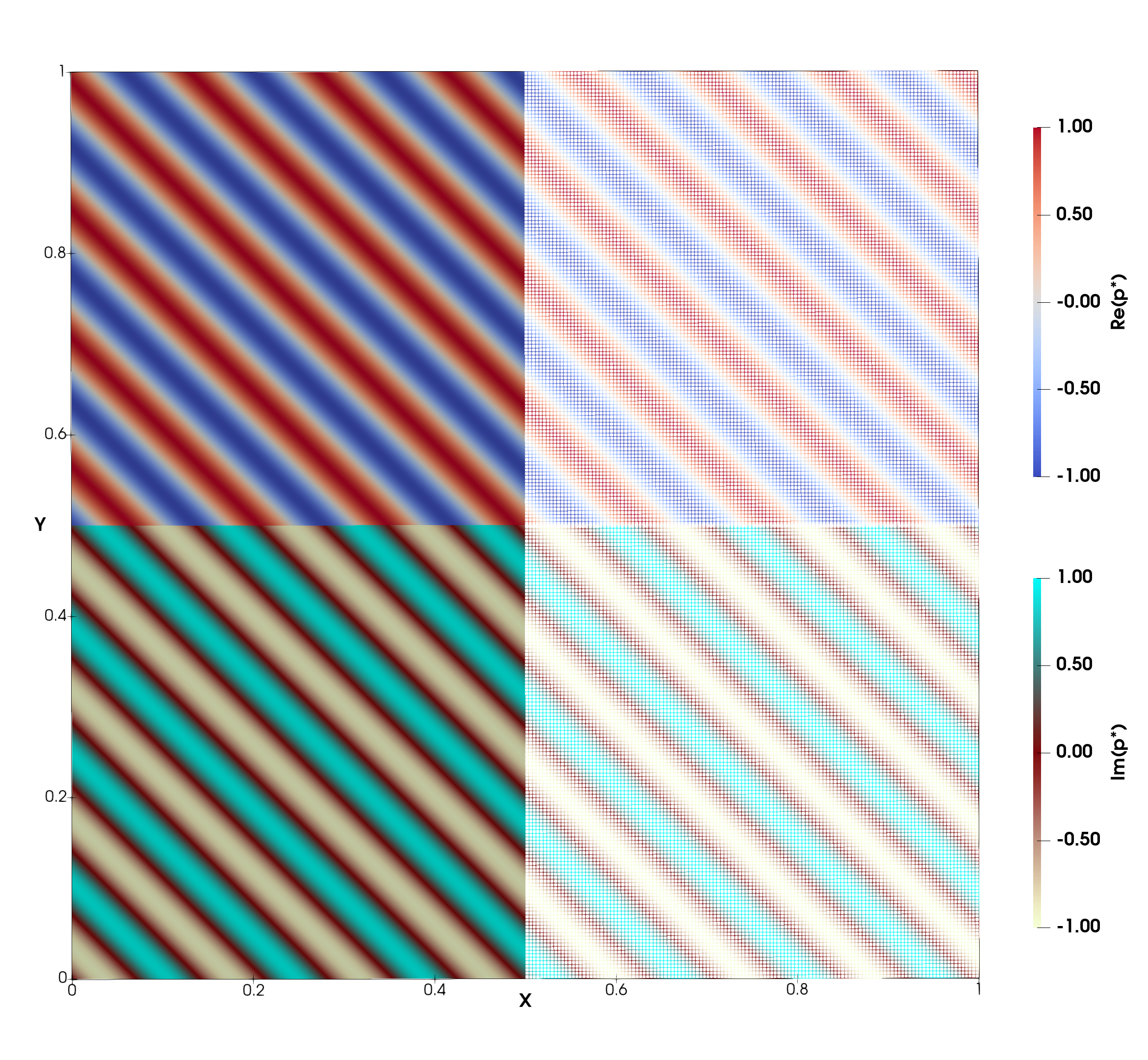
Convergence

To validate that the code falls back on the analytical solution of the plane wave with the expected order, we did a convergence plot for all the different fields which are presented below. As expected for degree \(p=2\) polynomial DGQ element in the interior, all fields converge to order 3. On the faces, it is expected that we lose half an order compared to the interior and that is what we observe for the normal velocity component. However, the pressure skeleton unknowns are associated with the trace of Q elements and for the same sequence of energy spaces the Q elements are one degree higher than the DGQ element. It follows that for DGQ of order 2 as used here, the corresponding Q element would be order 3 so the trace of those elements should converge with a slope of 3.5 as observed.
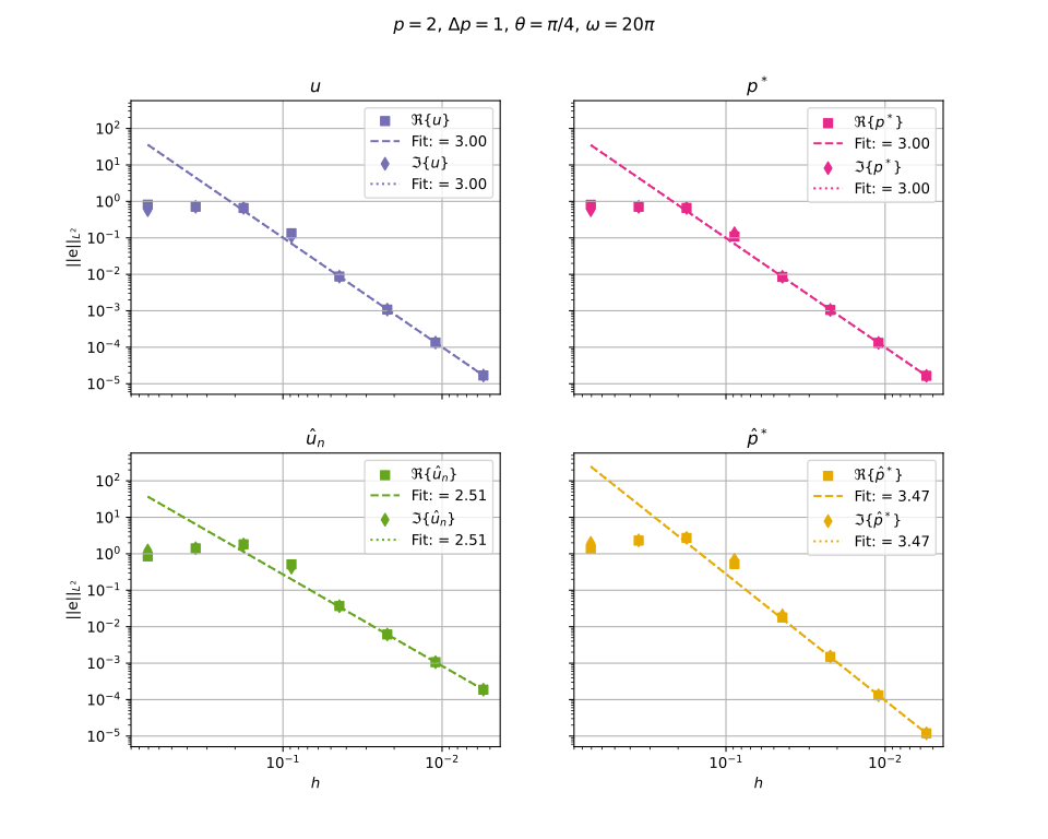
Linear solver iterations

In time-harmonic problems, the number of iterations to solve the system increases as the resolution of the wave increases (there are more dofs in the linear system). The DPG method is no exception to this. To show this, we recorded the number of iterations as we refined the mesh for 3 different angular frequencies and we present the result in the last figure below. In it, we show the number of iterations as a function of the number of dofs along with the total error of the interior fields. From it, we can see that the error does not start converging until the Nyquist criterion is respected, which requires the spatial discretization to resolve the wave with at least two points per wavelength. At that point there is a jump in the number of iterations to achieve convergence. After that the number of iterations approximately doubles each time we double the resolution. Nonetheless, because the DPG method enables the use of a Conjugate Gradient solver we are able to obtain a solution even for high frequencies without exceeding amounts of memory.

Possibilities for extension

As an extension to get a feeling of the method, one could first try to implement the 3D version of the plane wave problem in the unit cube by adding a second angle \(\phi\). The analytical solution to this problem is also known and is described by:

\begin{align*} p^* & = e^{-i k (x \cos(\theta) \sin{\phi} + y \sin(\theta) \sin(\phi) + z \cos(\phi))}, \\ \mathbf{u} & = \frac{1}{c_s} \begin{pmatrix} \cos(\theta) \sin(\phi) \\ \sin(\theta) \sin(\phi) \\ \cos(\phi) \end{pmatrix} e^{-i k (x \cos(\theta) \sin{\phi} + y \sin(\theta) \sin(\phi) + z \cos(\phi))}. \end{align*}

Another interesting extension would be to reconstruct the residual \(\Psi^r\) when the solutions on the faces and interior dofs are known and use it to build an error estimator that can be utilized for adaptive hp-refinement [199]. Finally, if one is interested more specifically in time-harmonic problems, the implementation of an adequate preconditioner to improve the convergence of the linear solver would remedy one of the inherent difficulties for this type of problem as stated by O. Ernst and M. J. Gander [89].

The plain program

/* ------------------------------------------------------------------------
*
* SPDX-License-Identifier: LGPL-2.1-or-later
* Copyright (C) 2025 - 2026 by the deal.II authors
*
* This file is part of the deal.II library.
*
* Part of the source code is dual licensed under Apache-2.0 WITH
* LLVM-exception OR LGPL-2.1-or-later. Detailed license information
* governing the source code and code contributions can be found in
* LICENSE.md and CONTRIBUTING.md at the top level directory of deal.II.
*
* ------------------------------------------------------------------------
*/
#include <fstream>
#include <iostream>
const double pi = ::numbers::PI;
namespace Step100
{
using namespace dealii;
template <int dim>
class AnalyticalSolutionPressureReal : public Function<dim>
{
public:
AnalyticalSolutionPressureReal(const double wavenumber, const double theta)
: Function<dim>()
, wavenumber(wavenumber)
, theta(theta)
{}
virtual double value(const Point<dim> &p,
const unsigned int component) const override;
private:
const double wavenumber;
const double theta;
};
template <int dim>
double AnalyticalSolutionPressureReal<dim>::value(
const Point<dim> &p,
const unsigned int /*component*/) const
{
return std::cos(wavenumber *
(p[0] * std::cos(theta) + p[1] * std::sin(theta)));
}
template <int dim>
class AnalyticalSolutionPressureImag : public Function<dim>
{
public:
AnalyticalSolutionPressureImag(const double wavenumber, const double theta)
: Function<dim>()
, wavenumber(wavenumber)
{}
virtual double value(const Point<dim> &p,
const unsigned int component) const override;
private:
const double wavenumber;
const double theta;
};
template <int dim>
double AnalyticalSolutionPressureImag<dim>::value(
const Point<dim> &p,
const unsigned int /*component*/) const
{
return -std::sin(wavenumber *
(p[0] * std::cos(theta) + p[1] * std::sin(theta)));
}
template <int dim>
class AnalyticalSolutionVelocityReal : public TensorFunction<1, dim>
{
public:
AnalyticalSolutionVelocityReal(const double wavenumber, const double theta)
: TensorFunction<1, dim>()
, wavenumber(wavenumber)
{}
virtual Tensor<1, dim> value(const Point<dim> &p) const override;
private:
const double wavenumber;
const double theta;
};
template <int dim>
AnalyticalSolutionVelocityReal<dim>::value(const Point<dim> &p) const
{
AssertDimension(dim, 2);
Tensor<1, dim> return_value;
return_value[0] =
std::cos(theta) *
std::cos(wavenumber * (p[0] * std::cos(theta) + p[1] * std::sin(theta)));
return_value[1] =
std::sin(theta) *
std::cos(wavenumber * (p[0] * std::cos(theta) + p[1] * std::sin(theta)));
return return_value;
}
template <int dim>
class AnalyticalSolutionVelocityImag : public TensorFunction<1, dim>
{
public:
AnalyticalSolutionVelocityImag(const double wavenumber, const double theta)
: TensorFunction<1, dim>()
, wavenumber(wavenumber)
{}
virtual Tensor<1, dim> value(const Point<dim> &p) const override;
private:
const double wavenumber;
const double theta;
};
template <int dim>
AnalyticalSolutionVelocityImag<dim>::value(const Point<dim> &p) const
{
AssertDimension(dim, 2);
Tensor<1, dim> return_value;
return_value[0] =
std::cos(theta) *
-std::sin(wavenumber * (p[0] * std::cos(theta) + p[1] * std::sin(theta)));
return_value[1] =
std::sin(theta) *
-std::sin(wavenumber * (p[0] * std::cos(theta) + p[1] * std::sin(theta)));
return return_value;
}
template <int dim>
class BoundaryValues : public Function<dim>
{
public:
BoundaryValues(const double wavenumber, const double theta)
: Function<dim>(4)
, wavenumber(wavenumber)
{}
virtual double value(const Point<dim> &p,
const unsigned int component) const override;
private:
double wavenumber;
double theta;
};
template <int dim>
double BoundaryValues<dim>::value(const Point<dim> &p,
const unsigned int component) const
{
if (component == 0)
{
return -1 * (std::sin(theta) *
std::cos(wavenumber * p[0] * std::cos(theta)));
}
else if (component == 1)
{
return std::sin(theta) * std::sin(wavenumber * p[0] * std::cos(theta));
}
else if (component == 2)
{
return std::cos(wavenumber * p[1] * std::sin(theta));
}
else if (component == 3)
{
return -std::sin(wavenumber * p[1] * std::sin(theta));
}
else
{
AssertThrow(false, ExcMessage("Invalid component for BoundaryValues"));
return 0.0;
}
}
template <int dim>
class DPGHelmholtz
{
public:
DPGHelmholtz(const unsigned int degree,
const unsigned int delta_degree,
const double wavenumber,
const double theta);
void run();
private:
void setup_system();
void assemble_system(bool solve_interior);
void solve_linear_system_skeleton();
void refine_grid(unsigned int cycle);
void output_results(unsigned int cycle);
void calculate_L2_error();
Triangulation<dim> triangulation;
const FESystem<dim> fe_trial_interior;
DoFHandler<dim> dof_handler_trial_interior;
Vector<double> solution_interior;
const FESystem<dim> fe_trial_skeleton;
DoFHandler<dim> dof_handler_trial_skeleton;
Vector<double> solution_skeleton;
Vector<double> system_rhs;
SparsityPattern sparsity_pattern;
SparseMatrix<double> system_matrix;
const FESystem<dim> fe_test;
DoFHandler<dim> dof_handler_test;
ConvergenceTable error_table;
const double wavenumber;
const double theta;
const FEValuesExtractors::Vector extractor_u_real;
const FEValuesExtractors::Vector extractor_u_imag;
const FEValuesExtractors::Scalar extractor_p_real;
const FEValuesExtractors::Scalar extractor_p_imag;
const FEValuesExtractors::Scalar extractor_u_hat_real;
const FEValuesExtractors::Scalar extractor_u_hat_imag;
const FEValuesExtractors::Scalar extractor_p_hat_real;
const FEValuesExtractors::Scalar extractor_p_hat_imag;
};
template <int dim>
DPGHelmholtz<dim>::DPGHelmholtz(const unsigned int degree,
const unsigned int delta_degree,
double wavenumber,
double theta)
: fe_trial_interior(FE_DGQ<dim>(degree) ^ dim,
FE_DGQ<dim>(degree) ^ dim,
FE_DGQ<dim>(degree),
FE_DGQ<dim>(degree))
, dof_handler_trial_interior(triangulation)
, fe_trial_skeleton(FE_FaceQ<dim>(degree),
FE_FaceQ<dim>(degree),
FE_TraceQ<dim>(degree + 1),
FE_TraceQ<dim>(degree + 1))
, dof_handler_trial_skeleton(triangulation)
, fe_test(FE_RaviartThomas<dim>(degree + delta_degree),
FE_RaviartThomas<dim>(degree + delta_degree),
FE_Q<dim>(degree + delta_degree + 1),
FE_Q<dim>(degree + delta_degree + 1))
, dof_handler_test(triangulation)
, wavenumber(wavenumber)
, extractor_u_real(0)
, extractor_u_imag(dim)
, extractor_p_real(2 * dim)
, extractor_p_imag(2 * dim + 1)
, extractor_u_hat_real(0)
, extractor_u_hat_imag(1)
, extractor_p_hat_real(2)
, extractor_p_hat_imag(3)
{
static_assert(dim == 2, "This tutorial example only works for dim==2");
AssertThrow(delta_degree >= 1,
ExcMessage("The delta_degree needs to be at least 1."));
AssertThrow(wavenumber > 0, ExcMessage("The wavenumber must be positive."));
AssertThrow(theta >= 0 && theta <= pi / 2,
ExcMessage(
"The angle theta must be in the interval [0, pi/2]."));
}
template <int dim>
void DPGHelmholtz<dim>::setup_system()
{
dof_handler_trial_skeleton.distribute_dofs(fe_trial_skeleton);
dof_handler_trial_interior.distribute_dofs(fe_trial_interior);
dof_handler_test.distribute_dofs(fe_test);
std::cout << std::endl
<< "Number of dofs for the interior: "
<< dof_handler_trial_interior.n_dofs() << std::endl;
error_table.add_value("dofs_interior", dof_handler_trial_interior.n_dofs());
std::cout << "Number of dofs for the skeleton: "
<< dof_handler_trial_skeleton.n_dofs() << std::endl;
error_table.add_value("dofs_skeleton", dof_handler_trial_skeleton.n_dofs());
std::cout << "Number of dofs for the test space: "
<< dof_handler_test.n_dofs() << std::endl;
error_table.add_value("dofs_test", dof_handler_test.n_dofs());
constraints.clear();
DoFTools::make_hanging_node_constraints(dof_handler_trial_skeleton,
constraints);
const BoundaryValues<dim> boundary_values(wavenumber, theta);
VectorTools::interpolate_boundary_values(dof_handler_trial_skeleton,
boundary_values,
constraints,
fe_trial_skeleton.component_mask(
extractor_p_hat_real));
VectorTools::interpolate_boundary_values(dof_handler_trial_skeleton,
boundary_values,
constraints,
fe_trial_skeleton.component_mask(
extractor_p_hat_imag));
VectorTools::interpolate_boundary_values(dof_handler_trial_skeleton,
boundary_values,
constraints,
fe_trial_skeleton.component_mask(
extractor_u_hat_real));
VectorTools::interpolate_boundary_values(dof_handler_trial_skeleton,
boundary_values,
constraints,
fe_trial_skeleton.component_mask(
extractor_u_hat_imag));
constraints.close();
solution_skeleton.reinit(dof_handler_trial_skeleton.n_dofs());
system_rhs.reinit(dof_handler_trial_skeleton.n_dofs());
solution_interior.reinit(dof_handler_trial_interior.n_dofs());
DynamicSparsityPattern dsp(dof_handler_trial_skeleton.n_dofs());
DoFTools::make_sparsity_pattern(dof_handler_trial_skeleton,
dsp,
constraints,
false);
sparsity_pattern.copy_from(dsp);
system_matrix.reinit(sparsity_pattern);
}
template <int dim>
void DPGHelmholtz<dim>::assemble_system(const bool solve_interior)
{
const QGauss<dim> quadrature_formula(fe_test.degree + 1);
const QGauss<dim - 1> face_quadrature_formula(fe_test.degree + 1);
const unsigned int n_q_points = quadrature_formula.size();
const unsigned int n_face_q_points = face_quadrature_formula.size();
FEValues<dim> fe_values_trial_interior(fe_trial_interior,
quadrature_formula,
FEValues<dim> fe_values_test(fe_test,
quadrature_formula,
FEFaceValues<dim> fe_values_trial_skeleton(fe_trial_skeleton,
face_quadrature_formula,
FEFaceValues<dim> fe_face_values_test(fe_test,
face_quadrature_formula,
const unsigned int dofs_per_cell_test = fe_test.n_dofs_per_cell();
const unsigned int dofs_per_cell_trial_interior =
fe_trial_interior.n_dofs_per_cell();
const unsigned int dofs_per_cell_trial_skeleton =
fe_trial_skeleton.n_dofs_per_cell();
std::vector<Tensor<1, dim, std::complex<double>>> v(dofs_per_cell_test);
std::vector<Tensor<1, dim, std::complex<double>>> v_conj(
dofs_per_cell_test);
std::vector<std::complex<double>> div_v(dofs_per_cell_test);
std::vector<std::complex<double>> div_v_conj(dofs_per_cell_test);
std::vector<std::complex<double>> q(dofs_per_cell_test);
std::vector<std::complex<double>> q_conj(dofs_per_cell_test);
std::vector<Tensor<1, dim, std::complex<double>>> grad_q(
dofs_per_cell_test);
std::vector<Tensor<1, dim, std::complex<double>>> grad_q_conj(
dofs_per_cell_test);
std::vector<std::complex<double>> v_face_n(dofs_per_cell_test);
std::vector<std::complex<double>> v_face_n_conj(dofs_per_cell_test);
std::vector<std::complex<double>> q_face(dofs_per_cell_test);
std::vector<std::complex<double>> q_face_conj(dofs_per_cell_test);
std::vector<Tensor<1, dim, std::complex<double>>> u(
dofs_per_cell_trial_interior);
std::vector<std::complex<double>> p(dofs_per_cell_trial_interior);
std::vector<std::complex<double>> u_hat_n(dofs_per_cell_trial_skeleton);
std::vector<std::complex<double>> u_hat_n_conj(
dofs_per_cell_trial_skeleton);
std::vector<std::complex<double>> p_hat(dofs_per_cell_trial_skeleton);
std::vector<std::complex<double>> p_hat_conj(dofs_per_cell_trial_skeleton);
enum ShapeFunctionType : unsigned char
{
velocity_real = 1u << 0,
velocity_imag = 1u << 1,
pressure_real = 1u << 2,
pressure_imag = 1u << 3,
is_velocity = velocity_real | velocity_imag,
is_pressure = pressure_real | pressure_imag
};
std::vector<unsigned char> shape_function_type_test(dofs_per_cell_test);
std::vector<unsigned char> shape_function_type_trial_interior(
dofs_per_cell_trial_interior);
std::vector<unsigned char> shape_function_type_trial_skeleton(
dofs_per_cell_trial_skeleton);
LAPACKFullMatrix<double> G_matrix(dofs_per_cell_test, dofs_per_cell_test);
LAPACKFullMatrix<double> B_matrix(dofs_per_cell_test,
dofs_per_cell_trial_interior);
LAPACKFullMatrix<double> B_hat_matrix(dofs_per_cell_test,
dofs_per_cell_trial_skeleton);
LAPACKFullMatrix<double> D_matrix(dofs_per_cell_trial_skeleton,
dofs_per_cell_trial_skeleton);
Vector<double> g_vector(dofs_per_cell_trial_skeleton);
Vector<double> l_vector(dofs_per_cell_test);
LAPACKFullMatrix<double> M1_matrix(dofs_per_cell_trial_interior,
dofs_per_cell_trial_interior);
LAPACKFullMatrix<double> M2_matrix(dofs_per_cell_trial_interior,
dofs_per_cell_trial_skeleton);
LAPACKFullMatrix<double> M3_matrix(dofs_per_cell_trial_skeleton,
dofs_per_cell_trial_skeleton);
LAPACKFullMatrix<double> M4_matrix(dofs_per_cell_trial_interior,
dofs_per_cell_test);
LAPACKFullMatrix<double> M5_matrix(dofs_per_cell_trial_skeleton,
dofs_per_cell_test);
LAPACKFullMatrix<double> tmp_matrix(dofs_per_cell_trial_skeleton,
dofs_per_cell_trial_interior);
LAPACKFullMatrix<double> tmp_matrix2(dofs_per_cell_trial_skeleton,
dofs_per_cell_trial_skeleton);
LAPACKFullMatrix<double> tmp_matrix3(dofs_per_cell_trial_skeleton,
dofs_per_cell_test);
Vector<double> tmp_vector(dofs_per_cell_trial_interior);
FullMatrix<double> cell_matrix(dofs_per_cell_trial_skeleton,
dofs_per_cell_trial_skeleton);
Vector<double> cell_skeleton_rhs(dofs_per_cell_trial_skeleton);
std::vector<types::global_dof_index> local_dof_indices(
dofs_per_cell_trial_skeleton);
Vector<double> cell_interior_rhs(dofs_per_cell_trial_interior);
Vector<double> cell_interior_solution(dofs_per_cell_trial_interior);
Vector<double> cell_skeleton_solution(dofs_per_cell_trial_skeleton);
constexpr std::complex<double> imag(0., 1.);
const std::complex<double> iomega = imag * wavenumber;
const std::complex<double> iomega_conj = std::conj(iomega);
for (const auto &cell : dof_handler_trial_interior.active_cell_iterators())
{
fe_values_trial_interior.reinit(cell);
const typename DoFHandler<dim>::active_cell_iterator cell_test =
cell->as_dof_handler_iterator(dof_handler_test);
fe_values_test.reinit(cell_test);
const typename DoFHandler<dim>::active_cell_iterator cell_skeleton =
cell->as_dof_handler_iterator(dof_handler_trial_skeleton);
G_matrix = 0;
B_matrix = 0;
B_hat_matrix = 0;
D_matrix = 0;
g_vector = 0;
l_vector = 0;
M1_matrix = 0;
for (unsigned int q_point = 0; q_point < n_q_points; ++q_point)
{
const double JxW = fe_values_trial_interior.JxW(q_point);
for (unsigned int k : fe_values_test.dof_indices())
{
v[k] =
fe_values_test[extractor_u_real].value(k, q_point) +
imag * fe_values_test[extractor_u_imag].value(k, q_point);
v_conj[k] =
fe_values_test[extractor_u_real].value(k, q_point) -
imag * fe_values_test[extractor_u_imag].value(k, q_point);
div_v[k] =
fe_values_test[extractor_u_real].divergence(k, q_point) +
imag *
fe_values_test[extractor_u_imag].divergence(k, q_point);
div_v_conj[k] =
fe_values_test[extractor_u_real].divergence(k, q_point) -
imag *
fe_values_test[extractor_u_imag].divergence(k, q_point);
q[k] =
fe_values_test[extractor_p_real].value(k, q_point) +
imag * fe_values_test[extractor_p_imag].value(k, q_point);
q_conj[k] =
fe_values_test[extractor_p_real].value(k, q_point) -
imag * fe_values_test[extractor_p_imag].value(k, q_point);
grad_q[k] =
fe_values_test[extractor_p_real].gradient(k, q_point) +
imag * fe_values_test[extractor_p_imag].gradient(k, q_point);
grad_q_conj[k] =
fe_values_test[extractor_p_real].gradient(k, q_point) -
imag * fe_values_test[extractor_p_imag].gradient(k, q_point);
if (fe_test.shape_function_belongs_to(k, extractor_u_real))
shape_function_type_test[k] |= velocity_real;
if (fe_test.shape_function_belongs_to(k, extractor_u_imag))
shape_function_type_test[k] |= velocity_imag;
if (fe_test.shape_function_belongs_to(k, extractor_p_real))
shape_function_type_test[k] |= pressure_real;
if (fe_test.shape_function_belongs_to(k, extractor_p_imag))
shape_function_type_test[k] |= pressure_imag;
}
for (unsigned int k : fe_values_trial_interior.dof_indices())
{
u[k] =
fe_values_trial_interior[extractor_u_real].value(k, q_point) +
imag *
fe_values_trial_interior[extractor_u_imag].value(k,
q_point);
p[k] =
fe_values_trial_interior[extractor_p_real].value(k, q_point) +
imag *
fe_values_trial_interior[extractor_p_imag].value(k,
q_point);
if (fe_trial_interior.shape_function_belongs_to(
k, extractor_u_real))
shape_function_type_trial_interior[k] |= velocity_real;
if (fe_trial_interior.shape_function_belongs_to(
k, extractor_u_imag))
shape_function_type_trial_interior[k] |= velocity_imag;
if (fe_trial_interior.shape_function_belongs_to(
k, extractor_p_real))
shape_function_type_trial_interior[k] |= pressure_real;
if (fe_trial_interior.shape_function_belongs_to(
k, extractor_p_imag))
shape_function_type_trial_interior[k] |= pressure_imag;
}
for (const auto i : fe_values_test.dof_indices())
{
const unsigned char test_type_i = shape_function_type_test[i];
for (const auto j : fe_values_test.dof_indices())
{
const unsigned char test_type_j =
shape_function_type_test[j];
if ((test_type_i & is_velocity) &&
(test_type_j & is_velocity))
{
G_matrix(i, j) +=
(((v_conj[i] * v[j]) + (div_v_conj[i] * div_v[j]) +
(iomega_conj * v_conj[i] * iomega * v[j])) *
JxW)
.real();
}
else if ((test_type_i & is_velocity) &&
(test_type_j & is_pressure))
{
G_matrix(i, j) +=
(((iomega_conj * v_conj[i] * grad_q[j]) +
(div_v_conj[i] * iomega * q[j])) *
JxW)
.real();
}
else if ((test_type_i & is_pressure) &&
(test_type_j & is_velocity))
{
G_matrix(i, j) +=
(((grad_q_conj[i] * iomega * v[j]) +
(iomega_conj * q_conj[i] * div_v[j])) *
JxW)
.real();
}
else if ((test_type_i & is_pressure) &&
(test_type_j & is_pressure))
{
G_matrix(i, j) +=
(((q_conj[i] * q[j]) + (grad_q[j] * grad_q_conj[i]) +
(iomega_conj * q_conj[i] * iomega * q[j])) *
JxW)
.real();
}
}
for (const auto j : fe_values_trial_interior.dof_indices())
{
const unsigned char trial_type_j =
shape_function_type_trial_interior[j];
if ((test_type_i & is_velocity) &&
(trial_type_j & is_velocity))
{
B_matrix(i, j) +=
((v_conj[i] * iomega * u[j]) * JxW).real();
}
else if ((test_type_i & is_velocity) &&
(trial_type_j & is_pressure))
{
B_matrix(i, j) -= ((div_v_conj[i] * p[j]) * JxW).real();
}
else if ((test_type_i & is_pressure) &&
(trial_type_j & is_velocity))
{
B_matrix(i, j) -=
((grad_q_conj[i] * u[j]) * JxW).real();
}
else if ((test_type_i & is_pressure) &&
(trial_type_j & is_pressure))
{
B_matrix(i, j) +=
((q_conj[i] * iomega * p[j]) * JxW).real();
}
}
if (test_type_i & is_pressure)
{
double source_term = 0.0;
l_vector(i) += (q_conj[i] * source_term * JxW).real();
}
}
}
for (const auto &face : cell_skeleton->face_iterators())
{
fe_face_values_test.reinit(cell_test, face);
fe_values_trial_skeleton.reinit(cell_skeleton, face);
const auto face_no = cell->face_iterator_to_index(face);
const auto current_boundary_id = face->boundary_id();
const double kn_omega =
(current_boundary_id == 1) ?
std::cos(theta) :
((current_boundary_id == 3) ? std::sin(theta) : 1.);
for (unsigned int q_point = 0; q_point < n_face_q_points; ++q_point)
{
const Tensor<1, dim> normal =
fe_values_trial_skeleton.normal_vector(q_point);
const double JxW_face = fe_values_trial_skeleton.JxW(q_point);
for (unsigned int k : fe_face_values_test.dof_indices())
{
v_face_n[k] =
normal *
(fe_face_values_test[extractor_u_real].value(k, q_point) +
imag *
fe_face_values_test[extractor_u_imag].value(k,
q_point));
v_face_n_conj[k] =
normal *
(fe_face_values_test[extractor_u_real].value(k, q_point) -
imag *
fe_face_values_test[extractor_u_imag].value(k,
q_point));
q_face[k] =
fe_face_values_test[extractor_p_real].value(k, q_point) +
imag *
fe_face_values_test[extractor_p_imag].value(k, q_point);
q_face_conj[k] =
fe_face_values_test[extractor_p_real].value(k, q_point) -
imag *
fe_face_values_test[extractor_p_imag].value(k, q_point);
if (fe_test.shape_function_belongs_to(k, extractor_u_real))
shape_function_type_test[k] |= velocity_real;
if (fe_test.shape_function_belongs_to(k, extractor_u_imag))
shape_function_type_test[k] |= velocity_imag;
if (fe_test.shape_function_belongs_to(k, extractor_p_real))
shape_function_type_test[k] |= pressure_real;
if (fe_test.shape_function_belongs_to(k, extractor_p_imag))
shape_function_type_test[k] |= pressure_imag;
}
for (unsigned int k : fe_values_trial_skeleton.dof_indices())
{
u_hat_n[k] =
fe_values_trial_skeleton[extractor_u_hat_real].value(
k, q_point) +
imag * fe_values_trial_skeleton[extractor_u_hat_imag]
.value(k, q_point);
u_hat_n_conj[k] =
fe_values_trial_skeleton[extractor_u_hat_real].value(
k, q_point) -
imag * fe_values_trial_skeleton[extractor_u_hat_imag]
.value(k, q_point);
p_hat[k] =
fe_values_trial_skeleton[extractor_p_hat_real].value(
k, q_point) +
imag * fe_values_trial_skeleton[extractor_p_hat_imag]
.value(k, q_point);
p_hat_conj[k] =
fe_values_trial_skeleton[extractor_p_hat_real].value(
k, q_point) -
imag * fe_values_trial_skeleton[extractor_p_hat_imag]
.value(k, q_point);
if (fe_trial_skeleton.shape_function_belongs_to(
k, extractor_u_hat_real))
shape_function_type_trial_skeleton[k] |= velocity_real;
if (fe_trial_skeleton.shape_function_belongs_to(
k, extractor_u_hat_imag))
shape_function_type_trial_skeleton[k] |= velocity_imag;
if (fe_trial_skeleton.shape_function_belongs_to(
k, extractor_p_hat_real))
shape_function_type_trial_skeleton[k] |= pressure_real;
if (fe_trial_skeleton.shape_function_belongs_to(
k, extractor_p_hat_imag))
shape_function_type_trial_skeleton[k] |= pressure_imag;
}
for (const auto i : fe_face_values_test.dof_indices())
{
const unsigned char face_test_type_i =
shape_function_type_test[i];
if (current_boundary_id == 1 || current_boundary_id == 3)
{
for (const auto j : fe_face_values_test.dof_indices())
{
const unsigned char face_test_type_j =
shape_function_type_test[j];
if ((face_test_type_i & is_velocity) &&
(face_test_type_j & is_velocity))
{
G_matrix(i, j) +=
(v_face_n_conj[i] * v_face_n[j] * JxW_face)
.real();
}
else if ((face_test_type_i & is_velocity) &&
(face_test_type_j & is_pressure))
{
G_matrix(i, j) += (v_face_n_conj[i] * kn_omega *
q_face[j] * JxW_face)
.real();
}
else if ((face_test_type_i & is_pressure) &&
(face_test_type_j & is_velocity))
{
G_matrix(i, j) += (kn_omega * q_face_conj[i] *
v_face_n[j] * JxW_face)
.real();
}
else if ((face_test_type_i & is_pressure) &&
(face_test_type_j & is_pressure))
{
G_matrix(i, j) +=
(kn_omega * q_face_conj[i] * kn_omega *
q_face[j] * JxW_face)
.real();
}
}
}
for (const auto j : fe_values_trial_skeleton.dof_indices())
{
const unsigned char face_trial_type_j =
shape_function_type_trial_skeleton[j];
if ((face_test_type_i & is_velocity) &&
(face_trial_type_j & is_pressure))
{
B_hat_matrix(i, j) +=
((v_face_n_conj[i] * p_hat[j]) * JxW_face).real();
}
else if ((face_test_type_i & is_pressure) &&
(face_trial_type_j & is_velocity))
{
const unsigned int neighbor_cell_id =
face->at_boundary() ?
std::numeric_limits<unsigned int>::max() :
cell->neighbor(face_no)->active_cell_index();
const double flux_orientation =
neighbor_cell_id > cell->active_cell_index() ?
1. :
-1.;
B_hat_matrix(i, j) +=
(q_face_conj[i] * flux_orientation * u_hat_n[j] *
JxW_face)
.real();
}
}
}
if (current_boundary_id == 1 || current_boundary_id == 3)
{
const double flux_orientation = 1.;
for (const auto i : fe_values_trial_skeleton.dof_indices())
{
const unsigned char face_trial_type_i =
shape_function_type_trial_skeleton[i];
for (const auto j :
fe_values_trial_skeleton.dof_indices())
{
const unsigned char face_trial_type_j =
shape_function_type_trial_skeleton[j];
if ((face_trial_type_i & is_velocity) &&
(face_trial_type_j & is_velocity))
{
D_matrix(i, j) -=
(flux_orientation * u_hat_n_conj[i] *
flux_orientation * u_hat_n[j] * JxW_face)
.real();
}
else if ((face_trial_type_i & is_velocity) &&
(face_trial_type_j & is_pressure))
{
D_matrix(i, j) +=
(flux_orientation * u_hat_n_conj[i] *
kn_omega * p_hat[j] * JxW_face)
.real();
}
else if ((face_trial_type_i & is_pressure) &&
(face_trial_type_j & is_velocity))
{
D_matrix(i, j) +=
(kn_omega * p_hat_conj[i] * flux_orientation *
u_hat_n[j] * JxW_face)
.real();
}
else if ((face_trial_type_i & is_pressure) &&
(face_trial_type_j & is_pressure))
{
D_matrix(i, j) -=
(kn_omega * p_hat_conj[i] * kn_omega *
p_hat[j] * JxW_face)
.real();
}
}
double source_term = 0.;
if (face_trial_type_i & is_velocity)
{
g_vector(i) -=
(u_hat_n_conj[i] * source_term).real() * JxW_face;
}
else if (face_trial_type_i & is_pressure)
{
g_vector(i) +=
(kn_omega * p_hat_conj[i] * source_term).real() *
JxW_face;
}
}
}
}
}
G_matrix.invert();
B_matrix.Tmmult(M4_matrix, G_matrix);
B_hat_matrix.Tmmult(M5_matrix, G_matrix);
M4_matrix.mmult(M1_matrix, B_matrix);
M4_matrix.mmult(M2_matrix, B_hat_matrix);
M5_matrix.mmult(M3_matrix, B_hat_matrix);
M3_matrix.add(-1.0, D_matrix);
M1_matrix.invert();
if (solve_interior)
{
cell_skeleton->get_dof_values(solution_skeleton,
cell_skeleton_solution);
M2_matrix.vmult(tmp_vector, cell_skeleton_solution);
M4_matrix.vmult(cell_interior_rhs, l_vector);
cell_interior_rhs -= tmp_vector;
M1_matrix.vmult(cell_interior_solution, cell_interior_rhs);
cell->distribute_local_to_global(cell_interior_solution,
solution_interior);
}
else
{
M2_matrix.Tmmult(tmp_matrix, M1_matrix);
tmp_matrix.mmult(tmp_matrix2, M2_matrix);
tmp_matrix2.add(-1.0, M3_matrix);
tmp_matrix2 *= -1.0;
cell_matrix = tmp_matrix2;
tmp_matrix.mmult(tmp_matrix3, M4_matrix);
M5_matrix.add(-1.0, tmp_matrix3);
M5_matrix.vmult(cell_skeleton_rhs, l_vector);
cell_skeleton_rhs -= g_vector;
cell_skeleton->get_dof_indices(local_dof_indices);
constraints.distribute_local_to_global(cell_matrix,
cell_skeleton_rhs,
local_dof_indices,
system_matrix,
system_rhs);
}
}
}
template <int dim>
void DPGHelmholtz<dim>::solve_linear_system_skeleton()
{
std::cout << std::endl << "Solving the DPG system..." << std::endl;
SolverControl solver_control(100000, 1e-10 * system_rhs.l2_norm());
SolverCG<Vector<double>> solver(solver_control);
solver.solve(system_matrix,
solution_skeleton,
system_rhs,
constraints.distribute(solution_skeleton);
std::cout << " " << solver_control.last_step()
<< " CG iterations needed to obtain convergence. \n"
<< std::endl;
error_table.add_value("n_iter", solver_control.last_step());
}
template <int dim>
void DPGHelmholtz<dim>::output_results(const unsigned int cycle)
{
DataOut<dim> data_out;
data_out.attach_dof_handler(dof_handler_trial_interior);
std::vector<std::string> solution_interior_names;
for (unsigned int i = 0; i < dim; ++i)
{
solution_interior_names.emplace_back("velocity_real");
}
for (unsigned int i = 0; i < dim; ++i)
{
solution_interior_names.emplace_back("velocity_imag");
}
solution_interior_names.emplace_back("pressure_real");
solution_interior_names.emplace_back("pressure_imag");
std::vector<DataComponentInterpretation::DataComponentInterpretation>
data_component_interpretation;
for (unsigned int i = 0; i < dim; ++i)
{
data_component_interpretation.push_back(
}
for (unsigned int i = 0; i < dim; ++i)
{
data_component_interpretation.push_back(
}
data_component_interpretation.push_back(
data_out.add_data_vector(solution_interior,
solution_interior_names,
data_component_interpretation);
data_out.build_patches(fe_trial_interior.degree);
std::ofstream output("solution_planewave_square-" + std::to_string(cycle) +
".vtu");
data_out.write_vtu(output);
DataOutFaces<dim> data_out_faces(false);
data_out_faces.attach_dof_handler(dof_handler_trial_skeleton);
std::vector<std::string> solution_skeleton_names;
solution_skeleton_names.emplace_back("velocity_hat_real");
solution_skeleton_names.emplace_back("velocity_hat_imag");
solution_skeleton_names.emplace_back("pressure_hat_real");
solution_skeleton_names.emplace_back("pressure_hat_imag");
std::vector<DataComponentInterpretation::DataComponentInterpretation>
data_component_interpretation_skeleton(
data_out_faces.add_data_vector(solution_skeleton,
solution_skeleton_names,
data_component_interpretation_skeleton);
data_out_faces.build_patches(fe_trial_skeleton.degree);
std::ofstream output_face("solution_face_planewave_square-" +
std::to_string(cycle) + ".vtu");
data_out_faces.write_vtu(output_face);
}
template <int dim>
void DPGHelmholtz<dim>::calculate_L2_error()
{
QGauss<dim> quadrature_formula(fe_test.degree + 1);
FEValues<dim> fe_values_trial_interior(fe_trial_interior,
quadrature_formula,
const QGauss<dim - 1> face_quadrature_formula(fe_test.degree + 1);
FEFaceValues<dim> fe_values_trial_skeleton(fe_trial_skeleton,
face_quadrature_formula,
const unsigned int n_q_points = quadrature_formula.size();
const unsigned int n_face_q_points = face_quadrature_formula.size();
double L2_error_p_real = 0;
double L2_error_p_imag = 0;
double L2_error_p_hat_real = 0;
double L2_error_p_hat_imag = 0;
double L2_error_u_real = 0;
double L2_error_u_imag = 0;
double L2_error_u_hat_real = 0;
double L2_error_u_hat_imag = 0;
std::vector<Tensor<1, dim>> local_u_real(n_q_points);
std::vector<Tensor<1, dim>> local_u_imag(n_q_points);
std::vector<double> local_p_real(n_q_points);
std::vector<double> local_p_imag(n_q_points);
std::vector<double> local_u_hat_real(n_face_q_points);
std::vector<double> local_u_hat_imag(n_face_q_points);
std::vector<double> local_p_hat_real(n_face_q_points);
std::vector<double> local_p_hat_imag(n_face_q_points);
const AnalyticalSolutionPressureReal<dim> analytical_solution_p_real(
wavenumber, theta);
const AnalyticalSolutionPressureImag<dim> analytical_solution_p_imag(
wavenumber, theta);
const AnalyticalSolutionVelocityReal<dim> analytical_solution_u_real(
wavenumber, theta);
const AnalyticalSolutionVelocityImag<dim> analytical_solution_u_imag(
wavenumber, theta);
for (const auto &cell : dof_handler_trial_interior.active_cell_iterators())
{
fe_values_trial_interior.reinit(cell);
fe_values_trial_interior[extractor_u_real].get_function_values(
solution_interior, local_u_real);
fe_values_trial_interior[extractor_u_imag].get_function_values(
solution_interior, local_u_imag);
fe_values_trial_interior[extractor_p_real].get_function_values(
solution_interior, local_p_real);
fe_values_trial_interior[extractor_p_imag].get_function_values(
solution_interior, local_p_imag);
const auto &quadrature_points =
fe_values_trial_interior.get_quadrature_points();
for (const unsigned int q_index :
fe_values_trial_interior.quadrature_point_indices())
{
const double JxW = fe_values_trial_interior.JxW(q_index);
const auto &position = quadrature_points[q_index];
L2_error_u_real += (local_u_real[q_index] -
analytical_solution_u_real.value(position))
.norm_square() *
JxW;
L2_error_u_imag += (local_u_imag[q_index] -
analytical_solution_u_imag.value(position))
.norm_square() *
JxW;
L2_error_p_real +=
std::pow((local_p_real[q_index] -
analytical_solution_p_real.value(position, 0)),
2) *
JxW;
L2_error_p_imag +=
std::pow((local_p_imag[q_index] -
analytical_solution_p_imag.value(position, 0)),
2) *
JxW;
}
const typename DoFHandler<dim>::active_cell_iterator cell_skeleton =
cell->as_dof_handler_iterator(dof_handler_trial_skeleton);
for (const auto &face : cell->face_iterators())
{
fe_values_trial_skeleton.reinit(cell_skeleton, face);
const auto face_no = cell_skeleton->face_iterator_to_index(face);
fe_values_trial_skeleton[extractor_u_hat_real].get_function_values(
solution_skeleton, local_u_hat_real);
fe_values_trial_skeleton[extractor_u_hat_imag].get_function_values(
solution_skeleton, local_u_hat_imag);
fe_values_trial_skeleton[extractor_p_hat_real].get_function_values(
solution_skeleton, local_p_hat_real);
fe_values_trial_skeleton[extractor_p_hat_imag].get_function_values(
solution_skeleton, local_p_hat_imag);
const auto &face_quadrature_points =
fe_values_trial_skeleton.get_quadrature_points();
for (const unsigned int &q_index :
fe_values_trial_skeleton.quadrature_point_indices())
{
const double JxW = fe_values_trial_skeleton.JxW(q_index);
const auto &position = face_quadrature_points[q_index];
const Tensor<1, dim> normal =
fe_values_trial_skeleton.normal_vector(q_index);
const unsigned int neighbor_cell_id =
face->at_boundary() ?
std::numeric_limits<unsigned int>::max() :
cell->neighbor(face_no)->active_cell_index();
if (neighbor_cell_id < cell->active_cell_index())
{
continue;
}
double u_hat_n_analytical_real =
normal * analytical_solution_u_real.value(position);
double u_hat_n_analytical_imag =
normal * analytical_solution_u_imag.value(position);
L2_error_u_hat_real +=
std::pow(std::abs(local_u_hat_real[q_index]) -
std::abs(u_hat_n_analytical_real),
2) *
JxW;
L2_error_u_hat_imag +=
std::pow(std::abs(local_u_hat_imag[q_index]) -
std::abs(u_hat_n_analytical_imag),
2) *
JxW;
L2_error_p_hat_real +=
std::pow((local_p_hat_real[q_index] -
analytical_solution_p_real.value(position, 0)),
2) *
JxW;
L2_error_p_hat_imag +=
std::pow((local_p_hat_imag[q_index] -
analytical_solution_p_imag.value(position, 0)),
2) *
JxW;
}
}
}
std::cout << "Velocity real part L2 error is : "
<< std::sqrt(L2_error_u_real) << std::endl;
std::cout << "Velocity imag part L2 error is : "
<< std::sqrt(L2_error_u_imag) << std::endl;
std::cout << "Pressure real part L2 error is : "
<< std::sqrt(L2_error_p_real) << std::endl;
std::cout << "Pressure imag part L2 error is : "
<< std::sqrt(L2_error_p_imag) << std::endl;
std::cout << "Velocity skeleton real part L2 error is : "
<< std::sqrt(L2_error_u_hat_real) << std::endl;
std::cout << "Velocity skeleton imag part L2 error is : "
<< std::sqrt(L2_error_u_hat_imag) << std::endl;
std::cout << "Pressure skeleton real part L2 error is : "
<< std::sqrt(L2_error_p_hat_real) << std::endl;
std::cout << "Pressure skeleton imag part L2 error is : "
<< std::sqrt(L2_error_p_hat_imag) << std::endl;
error_table.add_value("eL2_u_r", std::sqrt(L2_error_u_real));
error_table.add_value("eL2_u_i", std::sqrt(L2_error_u_imag));
error_table.add_value("eL2_p_r", std::sqrt(L2_error_p_real));
error_table.add_value("eL2_p_i", std::sqrt(L2_error_p_imag));
error_table.add_value("eL2_u_hat_r", std::sqrt(L2_error_u_hat_real));
error_table.add_value("eL2_u_hat_i", std::sqrt(L2_error_u_hat_imag));
error_table.add_value("eL2_p_hat_r", std::sqrt(L2_error_p_hat_real));
error_table.add_value("eL2_p_hat_i", std::sqrt(L2_error_p_hat_imag));
}
template <int dim>
void DPGHelmholtz<dim>::refine_grid(const unsigned int cycle)
{
if (cycle == 0)
{
const Point<dim> p1{0., 0.};
const Point<dim> p2{1., 1.};
std::vector<unsigned int> repetitions({2, 2});
triangulation, repetitions, p1, p2, true);
triangulation.refine_global(0);
}
else
{
triangulation.refine_global();
}
std::cout << "Number of active cells: " << triangulation.n_active_cells()
<< std::endl;
error_table.add_value("cycle", cycle);
error_table.add_value("n_cells", triangulation.n_active_cells());
error_table.add_value("cell_size",
GridTools::maximal_cell_diameter<dim>(triangulation));
}
template <int dim>
void DPGHelmholtz<dim>::run()
{
for (unsigned int cycle = 0; cycle < 8; ++cycle)
{
std::cout << "===========================================" << std::endl
<< "Cycle " << cycle << ':' << std::endl;
refine_grid(cycle);
setup_system();
assemble_system(false);
solve_linear_system_skeleton();
assemble_system(true);
calculate_L2_error();
output_results(cycle);
}
error_table.evaluate_convergence_rates(
"eL2_u_r", "n_cells", ConvergenceTable::reduction_rate_log2);
error_table.evaluate_convergence_rates(
"eL2_u_i", "n_cells", ConvergenceTable::reduction_rate_log2);
error_table.evaluate_convergence_rates(
"eL2_p_r", "n_cells", ConvergenceTable::reduction_rate_log2);
error_table.evaluate_convergence_rates(
"eL2_p_i", "n_cells", ConvergenceTable::reduction_rate_log2);
error_table.evaluate_convergence_rates(
"eL2_u_hat_r", "n_cells", ConvergenceTable::reduction_rate_log2);
error_table.evaluate_convergence_rates(
"eL2_u_hat_i", "n_cells", ConvergenceTable::reduction_rate_log2);
error_table.evaluate_convergence_rates(
"eL2_p_hat_r", "n_cells", ConvergenceTable::reduction_rate_log2);
error_table.evaluate_convergence_rates(
"eL2_p_hat_i", "n_cells", ConvergenceTable::reduction_rate_log2);
std::cout << "===========================================" << std::endl;
std::cout << "Convergence table:" << std::endl;
error_table.write_text(std::cout);
}
} // End of namespace Step100
int main()
{
const unsigned int dim = 2;
try
{
const int degree = 2;
const int delta_degree = 1;
const double wavenumber = 20 * pi;
const double theta = pi / 4.;
std::cout << "===========================================" << std::endl
<< "Trial order: " << degree << std::endl
<< "Test order: " << delta_degree + degree << std::endl
<< "===========================================" << std::endl
<< std::endl;
Step100::DPGHelmholtz<dim> dpg_helmholtz(degree,
delta_degree,
wavenumber,
theta);
dpg_helmholtz.run();
std::cout << std::endl;
}
catch (std::exception &exc)
{
std::cerr << std::endl
<< std::endl
<< "----------------------------------------------------"
<< std::endl;
std::cerr << "Exception on processing: " << std::endl
<< exc.what() << std::endl
<< "Aborting!" << std::endl
<< "----------------------------------------------------"
<< std::endl;
return 1;
}
catch (...)
{
std::cerr << std::endl
<< std::endl
<< "----------------------------------------------------"
<< std::endl;
std::cerr << "Unknown exception!" << std::endl
<< "Aborting!" << std::endl
<< "----------------------------------------------------"
<< std::endl;
return 1;
}
return 0;
}
void write_vtu(std::ostream &out) const
void add_data_vector(const VectorType &data, const std::vector< std::string > &names, const DataVectorType type=type_automatic, const std::vector< DataComponentInterpretation::DataComponentInterpretation > &data_component_interpretation={})
virtual void build_patches(const unsigned int n_subdivisions=0)
Definition data_out.cc:1060
void reinit(const Triangulation< dim, spacedim > &tria)
void cell_matrix(FullMatrix< double > &M, const FEValuesBase< dim > &fe, const FEValuesBase< dim > &fetest, const ArrayView< const std::vector< double > > &velocity, const double factor=1.)
Definition advection.h:72
void quadrature_points(const Triangulation< dim, spacedim > &triangulation, const Quadrature< dim > &quadrature, const std::vector< std::vector< BoundingBox< spacedim > > > &global_bounding_boxes, ParticleHandler< dim, spacedim > &particle_handler, const Mapping< dim, spacedim > &mapping=(ReferenceCells::get_hypercube< dim >() .template get_default_linear_mapping< spacedim >()), const std::vector< std::vector< double > > &properties={})
void run(const Iterator &begin, const std_cxx20::type_identity_t< Iterator > &end, Worker worker, Copier copier, const ScratchData &sample_scratch_data, const CopyData &sample_copy_data, const unsigned int queue_length, const unsigned int chunk_size)