 |
Reference documentation for deal.II version 9.3.3
|
 |
Reference documentation for deal.II version 9.3.3
|
This tutorial depends on step-51.
This program was contributed by Zhuoran Wang. Some more information about this program, as well as more numerical results, are presented in [118] .
This tutorial program presents an implementation of the "weak Galerkin" finite element method for the Poisson equation. In some sense, the motivation for considering this method starts from the same point as in step-51: We would like to consider discontinuous shape functions, but then need to address the fact that the resulting problem has a much larger number of degrees of freedom compared to the usual continuous Galerkin method (because, for example, each vertex carries as many degrees of freedom as there are adjacent cells). We also have to address the fact that, unlike in the continuous Galerkin method, every degree of freedom on one cell couples with all of the degrees of freedom on each of its face neighbor cells. Consequently, the matrix one gets from the "traditional" discontinuous Galerkin methods are both large and relatively dense.
Both the hybridized discontinuous Galerkin method (HDG) in step-51 and the weak Galerkin (WG) method in this tutorial address the issue of coupling by introducing additional degrees of freedom whose shape functions only live on a face between cells (i.e., on the "skeleton" of the mesh), and which therefore "insulate" the degrees of freedom on the adjacent cells from each other: cell degrees of freedom only couple with other cell degrees of freedom on the same cell, as well as face degrees of freedom, but not with cell degrees of freedom on neighboring cells. Consequently, the coupling of shape functions for these cell degrees of freedom indeed couple on exactly one cell and the degrees of freedom defined on its faces.
For a given equation, say the second order Poisson equation, the difference between the HDG and the WG method is how precisely one formulates the problem that connects all of these different shape functions. (Indeed, for some WG and HDG formulation, it is possible to show that they are equivalent.) The HDG does things by reformulating second order problems in terms of a system of first order equations and then conceptually considers the face degrees of freedom to be "fluxes" of this first order system. In contrast, the WG method keeps things in second order form and considers the face degrees of freedom as of the same type as the primary solution variable, just restricted to the lower-dimensional faces. For the purposes of the equation, one then needs to somehow "extend" these shape functions into the interior of the cell when defining what it means to apply a differential operator to them. Compared to the HDG, the method has the advantage that it does not lead to a proliferation of unknowns due to rewriting the equation as a first-order system, but it is also not quite as easy to implement. However, as we will see in the following, this additional effort is not prohibitive.
Weak Galerkin Finite Element Methods (WGFEMs) use discrete weak functions to approximate scalar unknowns, and discrete weak gradients to approximate classical gradients. The method was originally introduced by Junping Wang and Xiu Ye in the paper A weak Galerkin finite element method for second order elliptic problems, J. Comput. Appl. Math., 103-115, 2013. Compared to the continuous Galerkin method, the weak Galerkin method satisfies important physical properties, namely local mass conservation and bulk normal flux continuity. It results in a SPD linear system, and optimal convergence rates can be obtained with mesh refinement.
This program solves the Poisson equation using the weak Galerkin finite element method:
\begin{align*} \nabla \cdot \left( -\mathbf{K} \nabla p \right) &= f, \qquad \mathbf{x} \in \Omega, \\ p &= p_D,\qquad \mathbf{x} \in \Gamma^D, \\ \mathbf{u} \cdot \mathbf{n} &= u_N, \qquad \mathbf{x} \in \Gamma^N, \end{align*}
where \(\Omega \subset \mathbb{R}^n (n=2,3)\) is a bounded domain. In the context of the flow of a fluid through a porous medium, \(p\) is the pressure, \(\mathbf{K}\) is a permeability tensor, \(f\) is the source term, and \(p_D, u_N\) represent Dirichlet and Neumann boundary conditions. We can introduce a flux, \(\mathbf{u} = -\mathbf{K} \nabla p\), that corresponds to the Darcy velocity (in the way we did in step-20) and this variable will be important in the considerations below.
In this program, we will consider a test case where the exact pressure is \(p = \sin \left( \pi x\right)\sin\left(\pi y \right)\) on the unit square domain, with homogeneous Dirichelet boundary conditions and \(\mathbf{K}\) the identity matrix. Then we will calculate \(L_2\) errors of pressure, velocity, and flux.
The Poisson equation above has a solution \(p\) that needs to satisfy the weak formulation of the problem,
\begin{equation*} \mathcal{A}\left(p,q \right) = \mathcal{F} \left(q \right), \end{equation*}
for all test functions \(q\), where
\begin{equation*} \mathcal{A}\left(p,q\right) \dealcoloneq \int_\Omega \left(\mathbf{K} \nabla p\right) \cdot \nabla q \;\mathrm{d}x, \end{equation*}
and
\begin{equation*} \mathcal{F}\left(q\right) \dealcoloneq \int_\Omega f \, q \;\mathrm{d}x - \int_{\Gamma^N} u_N q \; \mathrm{d}x. \end{equation*}
Here, we have integrated by parts in the bilinear form, and we are evaluating the gradient of \(p,p\) in the interior and the values of \(q\) on the boundary of the domain. All of this is well defined because we assume that the solution is in \(H^1\) for which taking the gradient and evaluating boundary values are valid operations.
The idea of the weak Galerkin method is now to approximate the exact \(p\) solution with a discontinuous function \(p_h\). This function may only be discontinuous along interfaces between cells, and because we will want to evaluate this function also along interfaces, we have to prescribe not only what values it is supposed to have in the cell interiors but also its values along interfaces. We do this by saying that \(p_h\) is actually a tuple, \(p_h=(p^\circ,p^\partial)\), though it's really just a single function that is either equal to \(p^\circ(x)\) or \(p^\partial(x)\), depending on whether it is evaluated at a point \(x\) that lies in the cell interior or on cell interfaces.
We would then like to simply stick this approximation into the bilinear form above. This works for the case where we have to evaluate the test function \(q_h\) on the boundary (where we would simply take its interface part \(q_h^\partial\)) but we have to be careful with the gradient because that is only defined in cell interiors. Consequently, the weak Galerkin scheme for the Poisson equation is defined by
\begin{equation*} \mathcal{A}_h\left(p_h,q \right) = \mathcal{F} \left(q_h \right), \end{equation*}
for all discrete test functions \(q_h\), where
\begin{equation*} \mathcal{A}_h\left(p_h,q_h\right) \dealcoloneq \sum_{K \in \mathbb{T}} \int_K \mathbf{K} \nabla_{w,d} p_h \cdot \nabla_{w,d} q_h \;\mathrm{d}x, \end{equation*}
and
\begin{equation*} \mathcal{F}\left(q_h\right) \dealcoloneq \sum_{K \in \mathbb{T}} \int_K f \, q_h^\circ \;\mathrm{d}x - \sum_{\gamma \in \Gamma_h^N} \int_\gamma u_N q_h^\partial \;\mathrm{d}x, \end{equation*}
The key point is that here, we have replaced the gradient \(\nabla p_h\) by the discrete weak gradient operator \(\nabla_{w,d} p_h\) that makes sense for our peculiarly defined approximation \(p_h\).
The question is then how that operator works. For this, let us first say how we think of the discrete approximation \(p_h\) of the pressure. As mentioned above, the "function" \(p_h\) actually consists of two parts: the values \(p_h^\circ\) in the interior of cells, and \(p_h^\partial\) on the interfaces. We have to define discrete (finite-dimensional) function spaces for both of these; in this program, we will use FE_DGQ for \(p_h^\circ\) as the space in the interior of cells (defined on each cell, but in general discontinuous along interfaces), and FE_FaceQ for \(p_h^\partial\) as the space on the interfaces.
Then let us consider just a single cell (because the integrals above are all defined cell-wise, and because the weak discrete gradient is defined cell-by-cell). The restriction of \(p_h\) to cell \(K\), \(p_h|_K\) then consists of the pair \((p_h^\circ|_K,p_h^\partial|_{\partial K})\). In essence, we can think of \(\nabla_{w,d} p_h\) of some function defined on \(K\) that approximates the gradient; in particular, if \(p_h|_K\) was the restriction of a differentiable function (to the interior and boundary of \(K\) – which would make it continuous between the interior and boundary), then \(\nabla_{w,d} p_h\) would simply be the exact gradient \(\nabla p_h\). But, since \(p_h|_K\) is not continuous between interior and boundary of \(K\), we need a more general definition; furthermore, we can not deal with arbitrary functions, and so require that \(\nabla_{w,d} p_h\) is also in a finite element space (which, since the gradient is a vector, has to be vector-valued, and because the weak gradient is defined on each cell separately, will also be discontinuous between cells).
The way this is done is to define this weak gradient operator \(\nabla_{w,d}|_K : DGQ_k(K) \times DGQ_r(\partial K) \rightarrow RT_s(K)\) (where \(RT_s(K)\) is the vector-valued Raviart-Thomas space of order \(s\) on cell \(K\)) in the following way:
\begin{equation*} \int_K \mathbf v_h \cdot (\nabla_{w,d} p_h) = -\int_K (\nabla \cdot \mathbf v_h) p_h^\circ +\int_{\partial K} (\mathbf v_h \cdot \mathbf n) p_h^\partial, \end{equation*}
for all test functions \(\mathbf v_h \in RT_s(K)\). This is, in essence, simply an application of the integration-by-parts formula. In other words, for a given \(p_h=(p^\circ_h,p^\partial_h)\), we need to think of \(\nabla_{w,d} p_h|_K\) as that Raviart-Thomas function of degree \(s\) for which the left hand side and right hand side are equal for all test functions.
A key point to make is then the following: While the usual gradient \(\nabla\) is a local operator that computes derivatives based simply on the value of a function at a point and its (infinitesimal) neighborhood, the weak discrete gradient \(\nabla_{w,d}\) does not have this property: It depends on the values of the function it is applied to on the entire cell, including the cell's boundary. Both are, however, linear operators as is clear from the definition of \(\nabla_{w,d}\) above, and that will allow us to represent \(\nabla_{w,d}\) via a matrix in the discussion below.
Since \(p_h\) is an element of a finite element space, we can expand it in a basis as we always do, i.e., we can write
\begin{equation*} p_h(\mathbf x) = \sum_j P_j \varphi_j(\mathbf x). \end{equation*}
Here, since \(p_h\) has two components (the interior and the interface components), the same must hold true for the basis functions \(\varphi_j(\mathbf x)\), which we can write as \(\varphi_j = (\varphi_j^\circ,\varphi_j^\partial)\). If you've followed the descriptions in step-8, step-20, and the documentation module on vector-valued problems, it will be no surprise that for some values of \(j\), \(\varphi_j^\circ\) will be zero, whereas for other values of \(j\), \(\varphi_j^\partial\) will be zero – i.e., shape functions will be of either one or the other kind. That is not important, here, however. What is important is that we need to wonder how we can represent \(\nabla_{w,d} \varphi_j\) because that is clearly what will appear in the problem when we want to implement the bilinear form
\begin{equation*} \mathcal{A}_h\left(p_h,q_h\right) = \sum_{K \in \mathbb{T}} \int_K \mathbf{K} \nabla_{w,d} p_h \cdot \nabla_{w,d} q_h \;\mathrm{d}x, \end{equation*}
The key point is that \(\nabla_{w,d} \varphi_j\) is known to be a member of the "broken" Raviart-Thomas space \(DGRT_s\). What this means is that we can represent (on each cell \(K\) separately)
\begin{equation*} \nabla_{w,d} \varphi_j|_K = \sum_k C_{jk}^K \mathbf v_k|_K \end{equation*}
where the functions \(\mathbf v_k \in DGRT_s\), and where \(C^K\) is a matrix of dimension
\begin{align*} \text{dim}\left(DGQ_k(K) \times DGQ_r(K)\right) &\times \text{dim}\left(RT_s(K)\right) \\ &= \left(\text{dim}(DGQ_k(K)) + \text{dim}(DGQ_r(K))\right) \times \text{dim}\left(RT_s(K)\right). \end{align*}
(That the weak discrete gradient can be represented as a matrix should not come as a surprise: It is a linear operator from one finite dimensional space to another finite dimensional space. If one chooses bases for both of these spaces, then every linear operator can of course be written as a matrix mapping the vector of expansion coefficients with regards to the basis of the domain space of the operator, to the vector of expansion coefficients with regards to the basis in the image space.)
Using this expansion, we can easily use the definition of the weak discrete gradient above to define what the matrix is going to be:
\begin{equation*} \int_K \mathbf v_i \cdot \left(\sum_k C_{jk}^K \mathbf v_k\right) = -\int_K (\nabla \cdot \mathbf v_i) \varphi_j^\circ +\int_{\partial K} (\mathbf v_i \cdot \mathbf n) \varphi_j^\partial, \end{equation*}
for all test functions \(\mathbf v_i \in DGRT_s\).
This clearly leads to a linear system of the form
\begin{equation*} \sum_k M_{ik}^K C_{jk}^K = G_{ij}^K \end{equation*}
with
\begin{equation*} M_{ik}^K = \int_K \mathbf v_i \cdot \mathbf v_k, \qquad\qquad G_{ij}^K = -\int_K (\nabla \cdot \mathbf v_i) \varphi_j^\circ +\int_{\partial K} (\mathbf v_i \cdot \mathbf n) \varphi_j^\partial, \end{equation*}
and consequently
\begin{equation*} \left(C^K\right)^T = \left(M^K\right)^{-1} G^K. \end{equation*}
(In this last step, we have assumed that the indices \(i,j,k\) only range over those degrees of freedom active on cell \(K\), thereby ensuring that the mass matrix on the space \(RT_s(K)\) is invertible.) Equivalently, using the symmetry of the matrix \(M\), we have that
\begin{equation*} C^K = \left(G^K\right)^{T} \left(M^K\right)^{-1}. \end{equation*}
Also worth pointing out is that the matrices \(C^K\) and \(G^K\) are of course not square but rectangular.
Having explained how the weak discrete gradient is defined, we can now come back to the question of how the linear system for the equation in question should be assembled. Specifically, using the definition of the bilinear form \({\cal A}_h\) shown above, we then need to compute the elements of the local contribution to the global matrix,
\begin{equation*} A^K_{ij} = \int_K \left({\mathbf K} \nabla_{w,d} \varphi_i\right) \cdot \nabla_{w,d} \varphi_j. \end{equation*}
As explained above, we can expand \(\nabla_{w,d} \varphi_i\) in terms of the Raviart-Thomas basis on each cell, and similarly for \(\nabla_{w,d} \varphi_j\):
\begin{equation*} A^K_{ij} = \int_K \left( {\mathbf K} \sum_k C_{ik}^K \mathbf v_k|_K \right) \cdot \sum_l C_{jl}^K \mathbf v_l|_K. \end{equation*}
By re-arranging sums, this yields the following expression:
\begin{equation*} A^K_{ij} = \sum_k \sum_l C_{ik}^K C_{jl}^K \int_K \left( {\mathbf K} \mathbf v_k|_K \right) \cdot \mathbf v_l|_K. \end{equation*}
So, if we have the matrix \(C^K\) for each cell \(K\), then we can easily compute the contribution \(A^K\) for cell \(K\) to the matrix \(A\) as follows:
\begin{equation*} A^K_{ij} = \sum_k \sum_l C_{ik}^K C_{jl}^K H^K_{kl} = \sum_k \sum_l C_{ik}^K H^K_{kl} C_{jl}^K = \left(C^K H^K (C^K)^T \right)_{ij}. \end{equation*}
Here,
\begin{equation*} H^K_{kl} = \int_K \left( {\mathbf K} \mathbf v_k|_K \right) \cdot \mathbf v_l|_K, \end{equation*}
which is really just the mass matrix on cell \(K\) using the Raviart-Thomas basis and weighting by the permeability tensor \(\mathbf K\). The derivation here then shows that the weak Galerkin method really just requires us to compute these \(C^K\) and \(H^K\) matrices on each cell \(K\), and then \(A^K = C^K H^K (C^K)^T\), which is easily computed. The code to be shown below does exactly this.
Having so computed the contribution \(A^K\) of cell \(K\) to the global matrix, all we have to do is to "distribute" these local contributions into the global matrix. How this is done is first shown in step-3 and step-4. In the current program, this will be facilitated by calling AffineConstraints::distribute_local_to_global().
A linear system of course also needs a right hand side. There is no difficulty associated with computing the right hand side here other than the fact that we only need to use the cell-interior part \(\varphi_i^\circ\) for each shape function \(\varphi_i\).
The discussions in the previous sections have given us a linear system that we can solve for the numerical pressure \(p_h\). We can use this to compute an approximation to the variable \(\mathbf u = -{\mathbf K}\nabla p\) that corresponds to the velocity with which the medium flows in a porous medium if this is the model we are trying to solve. This kind of step – computing a derived quantity from the solution of the discrete problem – is typically called "post-processing".
Here, instead of using the exact gradient of \(p_h\), let us instead use the discrete weak gradient of \(p_h\) to calculate the velocity on each element. As discussed above, on each element the gradient of the numerical pressure \(\nabla p\) can be approximated by discrete weak gradients \( \nabla_{w,d}\phi_i\):
\begin{equation*} \nabla_{w,d} p_h = \nabla_{w,d} \left(\sum_{i} P_i \phi_i\right) = \sum_{i} P_i \nabla_{w,d}\phi_i. \end{equation*}
On cell \(K\), the numerical velocity \( \mathbf{u}_h = -\mathbf{K} \nabla_{w,d}p_h\) can be written as
\begin{align*} \mathbf{u}_h &= -\mathbf{K} \nabla_{w,d} p_h = -\mathbf{K}\sum_{i} \sum_{j} P_i C^K_{ij}\mathbf{v}_j, \end{align*}
where \(C^K\) is the expansion matrix from above, and \(\mathbf{v}_j\) is the basis function of the \(RT\) space on a cell.
Unfortunately, \(\mathbf{K} \mathbf{v}_j\) may not be in the \(RT\) space (unless, of course, if \(\mathbf K\) is constant times the identity matrix). So, in order to represent it in a finite element program, we need to project it back into a finite dimensional space we can work with. Here, we will use the \(L_2\)-projection to project it back to the (broken) \(RT\) space.
We define the projection as \( \mathbf{Q}_h \left( \mathbf{K}\mathbf{v}_j \right) = \sum_{k} d_{jk}\mathbf{v}_k\) on each cell \(K\). For any \(j\), \(\left( \mathbf{Q}_h \left( \mathbf{Kv}_j \right),\mathbf{v}_k \right)_K = \left( \mathbf{Kv}_j,\mathbf{v}_k \right)_K.\) So, rather than the formula shown above, the numerical velocity on cell \(K\) instead becomes
\begin{equation*} \mathbf{u}_h = \mathbf{Q}_h \left( -\mathbf{K}\nabla_{w,d}p_h \right) = -\sum_i \sum_j P_i B^K_{ij}\mathbf{Q}_h \left( \mathbf{K}\mathbf{v}_j \right), \end{equation*}
and we have the following system to solve for the coefficients \(d_{jk}\):
\begin{equation*} \sum_j \left(\mathbf{v}_i,\mathbf{v}_j\right) d_{jk} = \left( \mathbf{Kv}_j,\mathbf{v}_k \right). \end{equation*}
In the implementation below, the matrix with elements \(
d_{jk}
\) is called cell_matrix_D, whereas the matrix with elements \(
\left( \mathbf{Kv}_j,\mathbf{v}_k \right)
\) is called cell_matrix_E.
Then the elementwise velocity is
\begin{equation*} \mathbf{u}_h = -\sum_{i} \sum_{j}P_ic_{ij}\sum_{k}d_{jk}\mathbf{v}_k = \sum_{k}- \left(\sum_{j} \sum_{i} P_ic_{ij}d_{jk} \right)\mathbf{v}_k, \end{equation*}
where \(-\sum_{j} \sum_{i} P_ic_{ij}d_{jk}\) is called cell_velocity in the code.
Using this velocity obtained by "postprocessing" the solution, we can define the \(L_2\)-errors of pressure, velocity, and flux by the following formulas:
\begin{align*} \|p-p_h^\circ\|^2 &= \sum_{K \in \mathbb{T}} \|p-p_h^\circ\|_{L_2(K)}^2, \\ \|\mathbf{u}-\mathbf{u}_h\|^2 &= \sum_{K \in \mathbb{T}} \|\mathbf{u}-\mathbf{u}_h\|_{L_2(K)^2}^d,\\ \|(\mathbf{u}-\mathbf{u}_h) \cdot \mathbf{n}\|^2 &= \sum_{K \in \mathbb{T}} \sum_{\gamma \subset \partial K} \frac{|K|}{|\gamma|} \|\mathbf{u} \cdot \mathbf{n} - \mathbf{u}_h \cdot \mathbf{n}\|_{L_2(\gamma)}^2, \end{align*}
where \(| K |\) is the area of the element, \(\gamma\) are faces of the element, \(\mathbf{n}\) are unit normal vectors of each face. The last of these norms measures the accuracy of the normal component of the velocity vectors over the interfaces between the cells of the mesh. The scaling factor \(|K|/|\gamma|\) is chosen so as to scale out the difference in the length (or area) of the collection of interfaces as the mesh size changes.
The first of these errors above is easily computed using VectorTools::integrate_difference. The others require a bit more work and are implemented in the code below.
This program is based on step-7, step-20 and step-51, so most of the following header files are familiar. We need the following, of which only the one that imports the FE_DGRaviartThomas class (namely, deal.II/fe/fe_dg_vector.h) is really new; the FE_DGRaviartThomas implements the "broken" Raviart-Thomas space discussed in the introduction:
Our first step, as always, is to put everything related to this tutorial program into its own namespace:
This is the main class of this program. We will solve for the numerical pressure in the interior and on faces using the weak Galerkin (WG) method, and calculate the \(L_2\) error of pressure. In the post-processing step, we will also calculate \(L_2\)-errors of the velocity and flux.
The structure of the class is not fundamentally different from that of previous tutorial programs, so there is little need to comment on the details with one exception: The class has a member variable fe_dgrt that corresponds to the "broken" Raviart-Thomas space mentioned in the introduction. There is a matching dof_handler_dgrt that represents a global enumeration of a finite element field created from this element, and a vector darcy_velocity that holds nodal values for this field. We will use these three variables after solving for the pressure to compute a postprocessed velocity field for which we can then evaluate the error and which we can output for visualization.
Next, we define the coefficient matrix \(\mathbf{K}\) (here, the identity matrix), Dirichlet boundary conditions, the right-hand side \(f = 2\pi^2 \sin(\pi x) \sin(\pi y)\), and the exact solution that corresponds to these choices for \(K\) and \(f\), namely \(p = \sin(\pi x) \sin(\pi y)\).
The class that implements the exact pressure solution has an oddity in that we implement it as a vector-valued one with two components. (We say that it has two components in the constructor where we call the constructor of the base Function class.) In the value() function, we do not test for the value of the component argument, which implies that we return the same value for both components of the vector-valued function. We do this because we describe the finite element in use in this program as a vector-valued system that contains the interior and the interface pressures, and when we compute errors, we will want to use the same pressure solution to test both of these components.
In this constructor, we create a finite element space for vector valued functions, which will here include the ones used for the interior and interface pressures, \(p^\circ\) and \(p^\partial\).
We generate a mesh on the unit square domain and refine it.
After we have created the mesh above, we distribute degrees of freedom and resize matrices and vectors. The only piece of interest in this function is how we interpolate the boundary values for the pressure. Since the pressure consists of interior and interface components, we need to make sure that we only interpolate onto that component of the vector-valued solution space that corresponds to the interface pressures (as these are the only ones that are defined on the boundary of the domain). We do this via a component mask object for only the interface pressures.
In the bilinear form, there is no integration term over faces between two neighboring cells, so we can just use DoFTools::make_sparsity_pattern to calculate the sparse matrix.
This function is more interesting. As detailed in the introduction, the assembly of the linear system requires us to evaluate the weak gradient of the shape functions, which is an element in the Raviart-Thomas space. As a consequence, we need to define a Raviart-Thomas finite element object, and have FEValues objects that evaluate it at quadrature points. We then need to compute the matrix \(C^K\) on every cell \(K\), for which we need the matrices \(M^K\) and \(G^K\) mentioned in the introduction.
A point that may not be obvious is that in all previous tutorial programs, we have always called FEValues::reinit() with a cell iterator from a DoFHandler. This is so that one can call functions such as FEValuesBase::get_function_values() that extract the values of a finite element function (represented by a vector of DoF values) on the quadrature points of a cell. For this operation to work, one needs to know which vector elements correspond to the degrees of freedom on a given cell – i.e., exactly the kind of information and operation provided by the DoFHandler class.
We could create a DoFHandler object for the "broken" Raviart-Thomas space (using the FE_DGRT class), but we really don't want to here: At least in the current function, we have no need for any globally defined degrees of freedom associated with this broken space, but really only need to reference the shape functions of such a space on the current cell. As a consequence, we use the fact that one can call FEValues::reinit() also with cell iterators into Triangulation objects (rather than DoFHandler objects). In this case, FEValues can of course only provide us with information that only references information about cells, rather than degrees of freedom enumerated on these cells. So we can't use FEValuesBase::get_function_values(), but we can use FEValues::shape_value() to obtain the values of shape functions at quadrature points on the current cell. It is this kind of functionality we will make use of below. The variable that will give us this information about the Raviart-Thomas functions below is then the fe_values_rt (and corresponding fe_face_values_rt) object.
Given this introduction, the following declarations should be pretty obvious:
Next, let us declare the various cell matrices discussed in the introduction:
We need FEValuesExtractors to access the interior and face component of the shape functions.
This finally gets us in position to loop over all cells. On each cell, we will first calculate the various cell matrices used to construct the local matrix – as they depend on the cell in question, they need to be re-computed on each cell. We need shape functions for the Raviart-Thomas space as well, for which we need to create first an iterator to the cell of the triangulation, which we can obtain by assignment from the cell pointing into the DoFHandler.
The first cell matrix we will compute is the mass matrix for the Raviart-Thomas space. Hence, we need to loop over all the quadrature points for the velocity FEValues object.
Next we take the inverse of this matrix by using FullMatrix::gauss_jordan(). It will be used to calculate the coefficient matrix \(C^K\) later. It is worth recalling later that cell_matrix_M actually contains the inverse of \(M^K\) after this call.
From the introduction, we know that the right hand side \(G^K\) of the equation that defines \(C^K\) is the difference between a face integral and a cell integral. Here, we approximate the negative of the contribution in the interior. Each component of this matrix is the integral of a product between a basis function of the polynomial space and the divergence of a basis function of the Raviart-Thomas space. These basis functions are defined in the interior.
Next, we approximate the integral on faces by quadrature. Each component is the integral of a product between a basis function of the polynomial space and the dot product of a basis function of the Raviart-Thomas space and the normal vector. So we loop over all the faces of the element and obtain the normal vector.
cell_matrix_C is then the matrix product between the transpose of \(G^K\) and the inverse of the mass matrix (where this inverse is stored in cell_matrix_M):
Finally we can compute the local matrix \(A^K\). Element \(A^K_{ij}\) is given by \(\int_{E} \sum_{k,l} C_{ik} C_{jl} (\mathbf{K} \mathbf{v}_k) \cdot \mathbf{v}_l \mathrm{d}x\). We have calculated the coefficients \(C\) in the previous step, and so obtain the following after suitably re-arranging the loops:
Next, we calculate the right hand side, \(\int_{K} f q \mathrm{d}x\):
The last step is to distribute components of the local matrix into the system matrix and transfer components of the cell right hand side into the system right hand side:
This step is rather trivial and the same as in many previous tutorial programs:
In this function, compute the velocity field from the pressure solution previously computed. The velocity is defined as \(\mathbf{u}_h = \mathbf{Q}_h \left( -\mathbf{K}\nabla_{w,d}p_h \right)\), which requires us to compute many of the same terms as in the assembly of the system matrix. There are also the matrices \(E^K,D^K\) we need to assemble (see the introduction) but they really just follow the same kind of pattern.
Computing the same matrices here as we have already done in the assemble_system() function is of course wasteful in terms of CPU time. Likewise, we copy some of the code from there to this function, and this is also generally a poor idea. A better implementation might provide for a function that encapsulates this duplicated code. One could also think of using the classic trade-off between computing efficiency and memory efficiency to only compute the \(C^K\) matrices once per cell during the assembly, storing them somewhere on the side, and re-using them here. (This is what step-51 does, for example, where the assemble_system() function takes an argument that determines whether the local matrices are recomputed, and a similar approach – maybe with storing local matrices elsewhere – could be adapted for the current program.)
In the introduction, we explained how to calculate the numerical velocity on the cell. We need the pressure solution values on each cell, coefficients of the Gram matrix and coefficients of the \(L_2\) projection. We have already calculated the global solution, so we will extract the cell solution from the global solution. The coefficients of the Gram matrix have been calculated when we assembled the system matrix for the pressures. We will do the same way here. For the coefficients of the projection, we do matrix multiplication, i.e., the inverse of the Gram matrix times the matrix with \((\mathbf{K} \mathbf{w}, \mathbf{w})\) as components. Then, we multiply all these coefficients and call them beta. The numerical velocity is the product of beta and the basis functions of the Raviart-Thomas space.
The component of this cell_matrix_E is the integral of \((\mathbf{K} \mathbf{w}, \mathbf{w})\). cell_matrix_M is the Gram matrix.
To compute the matrix \(D\) mentioned in the introduction, we then need to evaluate \(D=M^{-1}E\) as explained in the introduction:
Then we also need, again, to compute the matrix \(C\) that is used to evaluate the weak discrete gradient. This is the exact same code as used in the assembly of the system matrix, so we just copy it from there:
Finally, we need to extract the pressure unknowns that correspond to the current cell:
We are now in a position to compute the local velocity unknowns (with respect to the Raviart-Thomas space we are projecting the term \(-\mathbf K \nabla_{w,d} p_h\) into):
We compute Darcy velocity. This is same as cell_velocity but used to graph Darcy velocity.
This part is to calculate the \(L_2\) error of the pressure. We define a vector that holds the norm of the error on each cell. Next, we use VectorTool::integrate_difference() to compute the error in the \(L_2\) norm on each cell. However, we really only care about the error in the interior component of the solution vector (we can't even evaluate the interface pressures at the quadrature points because these are all located in the interior of cells) and consequently have to use a weight function that ensures that the interface component of the solution variable is ignored. This is done by using the ComponentSelectFunction whose arguments indicate which component we want to select (component zero, i.e., the interior pressures) and how many components there are in total (two).
In this function, we evaluate \(L_2\) errors for the velocity on each cell, and \(L_2\) errors for the flux on faces. The function relies on the compute_postprocessed_velocity() function having previous computed, which computes the velocity field based on the pressure solution that has previously been computed.
We are going to evaluate velocities on each cell and calculate the difference between numerical and exact velocities.
Having previously computed the postprocessed velocity, we here only have to extract the corresponding values on each cell and face and compare it to the exact values.
First compute the \(L_2\) error between the postprocessed velocity field and the exact one:
For reconstructing the flux we need the size of cells and faces. Since fluxes are calculated on faces, we have the loop over all four faces of each cell. To calculate the face velocity, we extract values at the quadrature points from the darcy_velocity which we have computed previously. Then, we calculate the squared velocity error in normal direction. Finally, we calculate the \(L_2\) flux error on the cell by appropriately scaling with face and cell areas and add it to the global error.
After adding up errors over all cells and faces, we take the square root and get the \(L_2\) errors of velocity and flux. These we output to screen.
We have two sets of results to output: the interior solution and the skeleton solution. We use DataOut to visualize interior results. The graphical output for the skeleton results is done by using the DataOutFaces class.
In both of the output files, both the interior and the face variables are stored. For the interface output, the output file simply contains the interpolation of the interior pressures onto the faces, but because it is undefined which of the two interior pressure variables you get from the two adjacent cells, it is best to ignore the interior pressure in the interface output file. Conversely, for the cell interior output file, it is of course impossible to show any interface pressures \(p^\partial\), because these are only available on interfaces and not cell interiors. Consequently, you will see them shown as an invalid value (such as an infinity).
For the cell interior output, we also want to output the velocity variables. This is a bit tricky since it lives on the same mesh but uses a different DoFHandler object (the pressure variables live on the dof_handler object, the Darcy velocity on the dof_handler_dgrt object). Fortunately, there are variations of the DataOut::add_data_vector() function that allow specifying which DoFHandler a vector corresponds to, and consequently we can visualize the data from both DoFHandler objects within the same file.
First attach the pressure solution to the DataOut object:
Then do the same with the Darcy velocity field, and continue with writing everything out into a file.
This is the final function of the main class. It calls the other functions of our class.
main functionThis is the main function. We can change the dimension here to run in 3d.
We run the program with a right hand side that will produce the solution \(p = \sin(\pi x) \sin(\pi y)\) and with homogeneous Dirichlet boundary conditions in the domain \(\Omega = (0,1)^2\). In addition, we choose the coefficient matrix in the differential operator \(\mathbf{K}\) as the identity matrix. We test this setup using \(\mbox{WG}(Q_0,Q_0;RT_{[0]})\), \(\mbox{WG}(Q_1,Q_1;RT_{[1]})\) and \(\mbox{WG}(Q_2,Q_2;RT_{[2]})\) element combinations, which one can select by using the appropriate constructor argument for the WGDarcyEquation object in main(). We will then visualize pressure values in interiors of cells and on faces. We want to see that the pressure maximum is around 1 and the minimum is around 0. With mesh refinement, the convergence rates of pressure, velocity and flux should then be around 1 for \(\mbox{WG}(Q_0,Q_0;RT_{[0]})\) , 2 for \(\mbox{WG}(Q_1,Q_1;RT_{[1]})\), and 3 for \(\mbox{WG}(Q_2,Q_2;RT_{[2]})\).
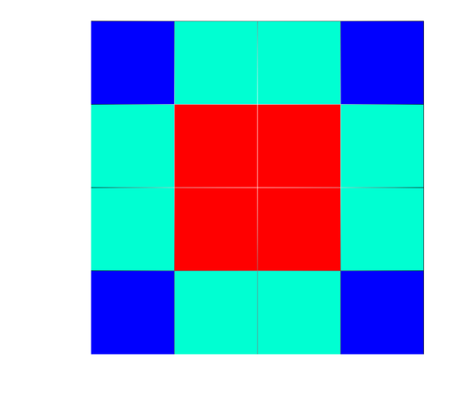
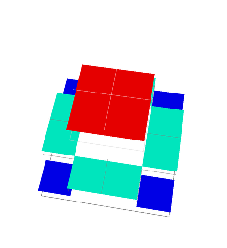
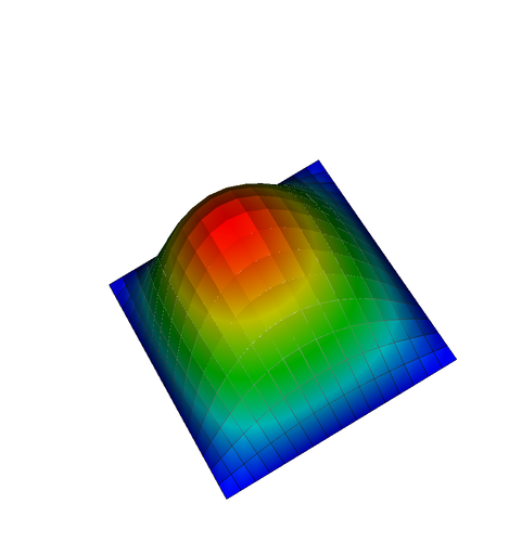
The following figures show interior pressures and face pressures using the \(\mbox{WG}(Q_0,Q_0;RT_{[0]})\) element. The mesh is refined 2 times (top) and 4 times (bottom), respectively. (This number can be adjusted in the make_grid() function.) When the mesh is coarse, one can see the face pressures \(p^\partial\) neatly between the values of the interior pressures \(p^\circ\) on the two adjacent cells.
 |  |
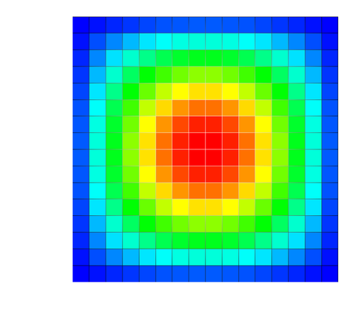 | 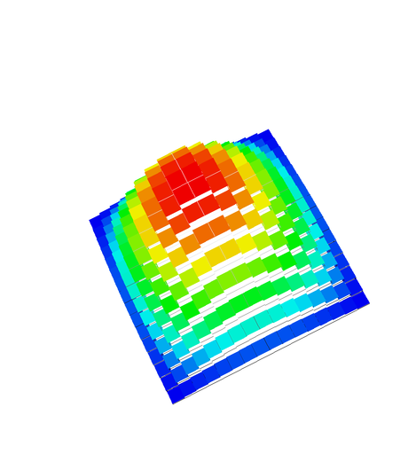 |
From the figures, we can see that with the mesh refinement, the maximum and minimum pressure values are approaching the values we expect. Since the mesh is a rectangular mesh and numbers of cells in each direction is even, we have symmetric solutions. From the 3d figures on the right, we can see that on \(\mbox{WG}(Q_0,Q_0;RT_{[0]})\), the pressure is a constant in the interior of the cell, as expected.
We run the code with differently refined meshes (chosen in the make_grid() function) and get the following convergence rates of pressure, velocity, and flux (as defined in the introduction).
| number of refinements | \(\|p-p_h^\circ\|\) | \(\|\mathbf{u}-\mathbf{u}_h\|\) | \(\|(\mathbf{u}-\mathbf{u}_h) \cdot \mathbf{n}\|\) |
|---|---|---|---|
| 2 | 1.587e-01 | 5.113e-01 | 7.062e-01 |
| 3 | 8.000e-02 | 2.529e-01 | 3.554e-01 |
| 4 | 4.006e-02 | 1.260e-01 | 1.780e-01 |
| 5 | 2.004e-02 | 6.297e-02 | 8.902e-02 |
| Conv.rate | 1.00 | 1.00 | 1.00 |
We can see that the convergence rates of \(\mbox{WG}(Q_0,Q_0;RT_{[0]})\) are around 1. This, of course, matches our theoretical expectations.
We can repeat the experiment from above using the next higher polynomial degree: The following figures are interior pressures and face pressures implemented using \(\mbox{WG}(Q_1,Q_1;RT_{[1]})\). The mesh is refined 4 times. Compared to the previous figures using \(\mbox{WG}(Q_0,Q_0;RT_{[0]})\), on each cell, the solution is no longer constant on each cell, as we now use bilinear polynomials to do the approximation. Consequently, there are 4 pressure values in one interior, 2 pressure values on each face.
 |  |
Compared to the corresponding image for the \(\mbox{WG}(Q_0,Q_0;RT_{[0]})\) combination, the solution is now substantially more accurate and, in particular so close to being continuous at the interfaces that we can no longer distinguish the interface pressures \(p^\partial\) from the interior pressures \(p^\circ\) on the adjacent cells.
The following are the convergence rates of pressure, velocity, and flux we obtain from using the \(\mbox{WG}(Q_1,Q_1;RT_{[1]})\) element combination:
| number of refinements | \(\|p-p_h^\circ\|\) | \(\|\mathbf{u}-\mathbf{u}_h\|\) | \(\|(\mathbf{u}-\mathbf{u}_h) \cdot \mathbf{n}\|\) |
|---|---|---|---|
| 2 | 1.613e-02 | 5.093e-02 | 7.167e-02 |
| 3 | 4.056e-03 | 1.276e-02 | 1.802e-02 |
| 4 | 1.015e-03 | 3.191e-03 | 4.512e-03 |
| 5 | 2.540e-04 | 7.979e-04 | 1.128e-03 |
| Conv.rate | 2.00 | 2.00 | 2.00 |
The convergence rates of \(WG(Q_1,Q_1;RT_{[1]})\) are around 2, as expected.
Let us go one polynomial degree higher. The following are interior pressures and face pressures implemented using \(WG(Q_2,Q_2;RT_{[2]})\), with mesh size \(h = 1/32\) (i.e., 5 global mesh refinement steps). In the program, we use data_out_face.build_patches(fe.degree) when generating graphical output (see the documentation of DataOut::build_patches()), which here implies that we divide each 2d cell interior into 4 subcells in order to provide a better visualization of the quadratic polynomials.
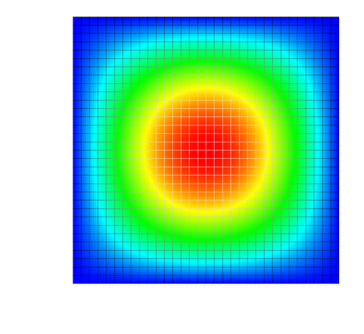 | 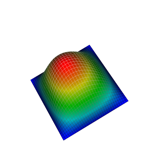 |
As before, we can generate convergence data for the \(L_2\) errors of pressure, velocity, and flux using the \(\mbox{WG}(Q_2,Q_2;RT_{[2]})\) combination:
| number of refinements | \(\|p-p_h^\circ\|\) | \(\|\mathbf{u}-\mathbf{u}_h\|\) | \(\|(\mathbf{u}-\mathbf{u}_h) \cdot \mathbf{n}\|\) |
|---|---|---|---|
| 2 | 1.072e-03 | 3.375e-03 | 4.762e-03 |
| 3 | 1.347e-04 | 4.233e-04 | 5.982e-04 |
| 4 | 1.685e-05 | 5.295e-05 | 7.487e-05 |
| 5 | 2.107e-06 | 6.620e-06 | 9.362e-06 |
| Conv.rate | 3.00 | 3.00 | 3.00 |
Once more, the convergence rates of \(\mbox{WG}(Q_2,Q_2;RT_{[2]})\) is as expected, with values around 3.