This tutorial depends on step-15, step-22.
This program was contributed by Liang Zhao and Timo Heister.
This material is based upon work partially supported by National Science Foundation grant DMS1522191 and the Computational Infrastructure in Geodynamics initiative (CIG), through the National Science Foundation under Award No. EAR-0949446 and The University of California-Davis.
- Note
- If you use this program as a basis for your own work, please consider citing it in your list of references. The initial version of this work was contributed to the deal.II project by the authors listed in the following citation:

Introduction
Navier Stokes Equations
In this tutorial we show how to solve the incompressible Navier Stokes equations (NSE) with Newton's method. The flow we consider here is assumed to be steady. In a domain \Omega \subset
\mathbb{R}^{d}, d=2,3, with a piecewise smooth boundary \partial \Omega, and a given force field \textbf{f}, we seek a velocity field \textbf{u} and a pressure field \textbf{p} satisfying
\begin{eqnarray*}
- \nu \Delta\textbf{u} + (\textbf{u} \cdot \nabla)\textbf{u} + \nabla p &=& \textbf{f}\\
- \nabla \cdot \textbf{u} &=& 0.
\end{eqnarray*}
Unlike the Stokes equations as discussed in step-22, the NSE are a nonlinear system of equations because of the convective term (\textbf{u} \cdot
\nabla)\textbf{u}. The first step of computing a numerical solution is to linearize the system and this will be done using Newton's method. A time-dependent problem is discussed in step-35, where the system is linearized using the solution from the last time step and no nonlinear solve is necessary.
Linearization of Navier-Stokes Equations
We define a nonlinear function whose root is a solution to the NSE by
\begin{eqnarray*}
F(\mathbf{u}, p) =
\begin{pmatrix}
- \nu \Delta\mathbf{u} + (\mathbf{u} \cdot \nabla)\mathbf{u} + \nabla p - \mathbf{f} \\
- \nabla \cdot \mathbf{u}
\end{pmatrix}.
\end{eqnarray*}
Assuming the initial guess is good enough to guarantee the convergence of Newton's iteration and denoting \textbf{x} = (\textbf{u}, p), Newton's iteration on a vector function can be defined as
\begin{eqnarray*}
\textbf{x}^{k+1} = \textbf{x}^{k} - (\nabla F(\textbf{x}^{k}))^{-1} F(\textbf{x}^{k}),
\end{eqnarray*}
where \textbf{x}^{k+1} is the approximate solution in step k+1, \textbf{x}^{k} represents the solution from the previous step, and \nabla
F(\textbf{x}^{k}) is the Jacobian matrix evaluated at \textbf{x}^{k}. A similar iteration can be found in step-15.
The Newton iteration formula implies the new solution is obtained by adding an update term to the old solution. Instead of evaluating the Jacobian matrix and taking its inverse, we consider the update term as a whole, that is
\begin{eqnarray*}
\delta \textbf{x}^{k} = - (\nabla F(\textbf{x}^{k}))^{-1} F(\textbf{x}^{k}),
\end{eqnarray*}
where \textbf{x}^{k+1}=\textbf{x}^{k}+\delta \textbf{x}^{k}.
We can find the update term by solving the system
\begin{eqnarray*}
\nabla F(\textbf{x}^{k}) \delta \textbf{x}^{k} = -F(\textbf{x}^{k}).
\end{eqnarray*}
Here, the left of the previous equation represents the directional gradient of F(\textbf{x}) along \delta
\textbf{x}^{k} at \textbf{x}^{k}. By definition, the directional gradient is given by
\begin{eqnarray*}
& &\nabla F(\mathbf{u}^{k}, p^{k}) (\delta \mathbf{u}^{k}, \delta p^{k}) \\
\\
&=& \lim_{\epsilon \to 0} \frac{1}{\epsilon}
\left(
F(\mathbf{u}^{k} + \epsilon \delta \mathbf{u}^{k},
p^{k} + \epsilon \nabla \delta p^{k})
- F(\mathbf{u}^{k}, p^{k})
\right)\\
\\
&=& \lim_{\epsilon \to 0} \frac{1}{\epsilon}
\begin{pmatrix}
- \epsilon \nu \Delta \delta \mathbf{u}^{k}
+ \epsilon \mathbf{u}^{k} \cdot \nabla \delta \mathbf{u}^{k}
+ \epsilon \delta \mathbf{u}^{k} \cdot \nabla \mathbf{u}^{k}
+ \epsilon^{2} \delta \mathbf{u}^{k} \cdot \nabla \delta \mathbf{u}^{k}
+ \epsilon \nabla \delta p^{k}\\
- \epsilon \nabla \cdot \delta \mathbf{u}^{k}
\end{pmatrix} \\
\\
&=& \begin{pmatrix}
- \nu \Delta \delta \mathbf{u}^{k}
+ \mathbf{u}^{k} \cdot \nabla \delta \mathbf{u}^{k}
+ \delta \mathbf{u}^{k} \cdot \nabla \mathbf{u}^{k}
+ \nabla \delta p^{k}\\
- \nabla \cdot \delta \mathbf{u}^{k}
\end{pmatrix}.
\end{eqnarray*}
Therefore, we arrive at the linearized system:
\begin{eqnarray*}
-\nu \Delta \delta \mathbf{u}^{k}
+ \mathbf{u}^{k} \cdot \nabla \delta \mathbf{u}^{k}
+ \delta \mathbf{u}^{k} \cdot \nabla \mathbf{u}^{k}
+ \nabla \delta p^{k}
= -F(\mathbf{x}^k), \\
-\nabla \cdot\delta \mathbf{u}^{k}
= \nabla \cdot \mathbf{u}^{k},
\end{eqnarray*}
where \textbf{u}^k and p^k are the solutions from the previous iteration. Additionally, the right hand side of the second equation is not zero since the discrete solution is not exactly divergence free (divergence free for the continuous solution). The right hand side here acts as a correction which leads the discrete solution of the velocity to be divergence free along Newton's iteration. In this linear system, the only unknowns are the update terms \delta \textbf{u}^{k} and \delta p^{k}, and we can use a similar strategy to the one used in step-22 (and derive the weak form in the same way).
Now, Newton's iteration can be used to solve for the update terms:
-
Initialization: Initial guess u_0 and p_0, tolerance \tau;
-
Linear solve to compute update term \delta\textbf{u}^{k} and \delta p^k;
-
Update the approximation: \textbf{u}^{k+1} = \textbf{u}^{k} + \delta\textbf{u}^{k} and p^{k+1} = p^{k} + \delta p^{k};
-
Check residual norm: E^{k+1} = \|F(\mathbf{u}^{k+1}, p^{k+1})\|:
-
If E^{k+1} \leq \tau, STOP.
-
If E^{k+1} > \tau, back to step 2.
Finding an Initial Guess
The initial guess needs to be close enough to the solution for Newton's method to converge; hence, finding a good starting value is crucial to the nonlinear solver.
When the viscosity \nu is large, a good initial guess can be obtained by solving the Stokes equation with viscosity \nu. While problem dependent, this works for \nu \geq 1/400 for the test problem considered here.
However, the convective term (\mathbf{u}\cdot\nabla)\mathbf{u} will be dominant if the viscosity is small, like 1/7500 in test case 2. In this situation, we use a continuation method to set up a series of auxiliary NSEs with viscosity approaching the one in the target NSE. Correspondingly, we create a sequence \{\nu_{i}\} with \nu_{n}= \nu, and accept that the solutions to two NSE with viscosity \nu_{i} and \nu_{i+1} are close if |\nu_{i} -
\nu_{i+1}| is small. Then we use the solution to the NSE with viscosity \nu_{i} as the initial guess of the NSE with \nu_{i+1}. This can be thought of as a staircase from the Stokes equations to the NSE we want to solve.
That is, we first solve a Stokes problem
\begin{eqnarray*}
-\nu_{1} \Delta \textbf{u} + \nabla p &=& \textbf{f}\\
-\nabla \cdot \textbf{u} &=& 0
\end{eqnarray*}
to get the initial guess for
\begin{eqnarray*}
-\nu_{1} \Delta \textbf{u} + (\textbf{u} \cdot \nabla)\textbf{u} + \nabla p &=& \textbf{f},\\
-\nabla \cdot \textbf{u} &=& 0,
\end{eqnarray*}
which also acts as the initial guess of the continuation method. Here \nu_{1} is relatively large so that the solution to the Stokes problem with viscosity \nu_{1} can be used as an initial guess for the NSE in Newton's iteration.
Then the solution to
\begin{eqnarray*}
-\nu_{i} \Delta \textbf{u} + (\textbf{u} \cdot \nabla)\textbf{u} + \nabla p &=& \textbf{f},\\
-\nabla \cdot \textbf{u} &=& 0.
\end{eqnarray*}
acts as the initial guess for
\begin{eqnarray*}
-\nu_{i+1} \Delta \textbf{u} + (\textbf{u} \cdot \nabla)\textbf{u} + \nabla p &=& \textbf{f},\\
-\nabla \cdot \textbf{u} &=& 0.
\end{eqnarray*}
This process is repeated with a sequence of viscosities \{\nu_i\} that is determined experimentally so that the final solution can used as a starting guess for the Newton iteration.
The Solver and Preconditioner
At each step of Newton's iteration, the problem results in solving a saddle point systems of the form
\begin{eqnarray*}
\begin{pmatrix}
A & B^{T} \\
B & 0
\end{pmatrix}
\begin{pmatrix}
U \\
P
\end{pmatrix}
=
\begin{pmatrix}
F \\
0
\end{pmatrix}.
\end{eqnarray*}
This system matrix has the same block structure as the one in step-22. However, the matrix A at the top left corner is not symmetric because of the nonlinear term. Instead of solving the above system, we can solve the equivalent system
\begin{eqnarray*}
\begin{pmatrix}
A + \gamma B^TW^{-1}B & B^{T} \\
B & 0
\end{pmatrix}
\begin{pmatrix}
U \\
P
\end{pmatrix}
=
\begin{pmatrix}
F \\
0
\end{pmatrix}
\end{eqnarray*}
with a parameter \gamma and an invertible matrix W. Here \gamma B^TW^{-1}B is the Augmented Lagrangian term; see [1] for details.
Denoting the system matrix of the new system by G and the right-hand side by b, we solve it iteratively with right preconditioning P^{-1} as GP^{-1}y = b, where
\begin{eqnarray*}
P^{-1} =
\begin{pmatrix}
\tilde{A} & B^T \\
0 & \tilde{S}
\end{pmatrix}^{-1}
\end{eqnarray*}
with \tilde{A} = A + \gamma B^TW^{-1}B and \tilde{S} is the corresponding Schur complement \tilde{S} = B^T \tilde{A}^{-1} B. We let W = M_p where M_p is the pressure mass matrix, then \tilde{S}^{-1} can be approximated by
\begin{eqnarray*}
\tilde{S}^{-1} \approx -(\nu+\gamma)M_p^{-1}.
\end{eqnarray*}
See [1] for details.
We decompose P^{-1} as
\begin{eqnarray*}
P^{-1} =
\begin{pmatrix}
\tilde{A}^{-1} & 0 \\
0 & I
\end{pmatrix}
\begin{pmatrix}
I & -B^T \\
0 & I
\end{pmatrix}
\begin{pmatrix}
I & 0 \\
0 & \tilde{S}^{-1}
\end{pmatrix}.
\end{eqnarray*}
Here two inexact solvers will be needed for \tilde{A}^{-1} and \tilde{S}^{-1}, respectively (see [1]). Since the pressure mass matrix is symmetric and positive definite, CG with ILU as a preconditioner is appropriate to use for \tilde{S}^{-1}. For simplicity, we use the direct solver UMFPACK for \tilde{A}^{-1}. The last ingredient is a sparse matrix-vector product with B^T. Instead of computing the matrix product in the augmented Lagrangian term in \tilde{A}, we assemble Grad-Div stabilization (\nabla \cdot \phi _{i}, \nabla \cdot \phi _{j}) \approx (B^T
M_p^{-1}B)_{ij}, as explained in [2].
Test Case
We use the lid driven cavity flow as our test case; see [3] for details. The computational domain is the unit square and the right-hand side is f=0. The boundary condition is
\begin{eqnarray*}
(u(x, y), v(x,y)) &=& (1,0) \qquad\qquad \textrm{if}\ y = 1 \\
(u(x, y), v(x,y)) &=& (0,0) \qquad\qquad \textrm{otherwise}.
\end{eqnarray*}
When solving this problem, the error consists of the nonlinear error (from Newton's iteration) and the discretization error (dependent on mesh size). The nonlinear part decreases with each Newton iteration and the discretization error reduces with mesh refinement. In this example, the solution from the coarse mesh is transferred to successively finer meshes and used as an initial guess. Therefore, the nonlinear error is always brought below the tolerance of Newton's iteration and the discretization error is reduced with each mesh refinement.
Inside the loop, we involve three solvers: one for \tilde{A}^{-1}, one for M_p^{-1} and one for Gx=b. The first two solvers are invoked in the preconditioner and the outer solver gives us the update term. Overall convergence is controlled by the nonlinear residual; as Newton's method does not require an exact Jacobian, we employ FGMRES with a relative tolerance of only 1e-4 for the outer linear solver. In fact, we use the truncated Newton solve for this system. As described in step-22, the inner linear solves are also not required to be done very accurately. Here we use CG with a relative tolerance of 1e-6 for the pressure mass matrix. As expected, we still see convergence of the nonlinear residual down to 1e-14. Also, we use a simple line search algorithm for globalization of the Newton method.
The cavity reference values for \mathrm{Re}=400 and \mathrm{Re}=7500 are from [4] and [5], respectively, where \mathrm{Re} is the Reynolds number and can be located at [8]. Here the viscosity is defined by 1/\mathrm{Re}. Even though we can still find a solution for \mathrm{Re}=10000 and the references contain results for comparison, we limit our discussion here to \mathrm{Re}=7500. This is because the solution is no longer stationary starting around \mathrm{Re}=8000 but instead becomes periodic, see [7] for details.
References
-
An Augmented Lagrangian-Based Approach to the Oseen Problem, M. Benzi and M. Olshanskii, SIAM J. SCI. COMPUT. 2006
-
Efficient augmented Lagrangian-type preconditioning for the Oseen problem using Grad-Div stabilization, Timo Heister and Gerd Rapin
-
http://www.cfd-online.com/Wiki/Lid-driven_cavity_problem
-
High-Re solution for incompressible flow using the Navier-Stokes Equations and a Multigrid Method, U. Ghia, K. N. Ghia, and C. T. Shin
-
Numerical solutions of 2-D steady incompressible driven cavity flow at high Reynolds numbers, E. Erturk, T.C. Corke and C. Gokcol
-
Implicit Weighted ENO Schemes for the Three-Dimensional Incompressible Navier-Stokes Equations, Yang et al, 1998
-
The 2D lid-driven cavity problem revisited, C. Bruneau and M. Saad, 2006
-
https://en.wikipedia.org/wiki/Reynolds_number
The commented program
Include files
As usual, we start by including some well-known files:
To transfer solutions between meshes, this file is included:
This file includes UMFPACK: the direct solver:
And the one for ILU preconditioner:
#include <fstream>
#include <iostream>
namespace Step57
{
The NavierStokesProblem class template
This class manages the matrices and vectors described in the introduction: in particular, we store a BlockVector for the current solution, current Newton update, and the line search update. We also store two AffineConstraints objects: one which enforces the Dirichlet boundary conditions and one that sets all boundary values to zero. The first constrains the solution vector while the second constraints the updates (i.e., we never update boundary values, so we force the relevant update vector values to be zero).
template <int dim>
class StationaryNavierStokes
{
public:
StationaryNavierStokes(const unsigned int degree);
void run(
const unsigned int refinement);
private:
void setup_dofs();
void initialize_system();
void assemble(
const bool initial_step,
const bool assemble_matrix);
void assemble_system(const bool initial_step);
void assemble_rhs(const bool initial_step);
void solve(const bool initial_step);
void refine_mesh();
void process_solution(unsigned int refinement);
void output_results(const unsigned int refinement_cycle) const;
void newton_iteration(const double tolerance,
const unsigned int max_n_line_searches,
const unsigned int max_n_refinements,
const bool is_initial_step,
const bool output_result);
void compute_initial_guess(double step_size);
double viscosity;
const unsigned int degree;
std::vector<types::global_dof_index> dofs_per_block;
};
void run(const Iterator &begin, const typename identity< Iterator >::type &end, Worker worker, Copier copier, const ScratchData &sample_scratch_data, const CopyData &sample_copy_data, const unsigned int queue_length, const unsigned int chunk_size)
long double gamma(const unsigned int n)
void assemble(const MeshWorker::DoFInfoBox< dim, DOFINFO > &dinfo, A *assembler)
const ::parallel::distributed::Triangulation< dim, spacedim > * triangulation
Boundary values and right hand side
In this problem we set the velocity along the upper surface of the cavity to be one and zero on the other three walls. The right hand side function is zero so we do not need to set the right hand side function in this tutorial. The number of components of the boundary function is dim+1. We will ultimately use VectorTools::interpolate_boundary_values to set boundary values, which requires the boundary value functions to have the same number of components as the solution, even if all are not used. Put another way: to make this function happy we define boundary values for the pressure even though we will never actually use them.
template <int dim>
class BoundaryValues :
public Function<dim>
{
public:
BoundaryValues()
{}
const unsigned int component) const override;
};
template <int dim>
double BoundaryValues<dim>::value(
const Point<dim> & p,
const unsigned int component) const
{
Assert(component < this->n_components,
if (component == 0 &&
std::abs(p[dim - 1] - 1.0) < 1
e-10)
return 1.0;
return 0;
}
virtual RangeNumberType value(const Point< dim > &p, const unsigned int component=0) const
static ::ExceptionBase & ExcIndexRange(int arg1, int arg2, int arg3)
#define Assert(cond, exc)
SymmetricTensor< 2, dim, Number > e(const Tensor< 2, dim, Number > &F)
::VectorizedArray< Number, width > abs(const ::VectorizedArray< Number, width > &)
BlockSchurPreconditioner for Navier Stokes equations
As discussed in the introduction, the preconditioner in Krylov iterative methods is implemented as a matrix-vector product operator. In practice, the Schur complement preconditioner is decomposed as a product of three matrices (as presented in the first section). The \tilde{A}^{-1} in the first factor involves a solve for the linear system \tilde{A}x=b. Here we solve this system via a direct solver for simplicity. The computation involved in the second factor is a simple matrix-vector multiplication. The Schur complement \tilde{S} can be well approximated by the pressure mass matrix and its inverse can be obtained through an inexact solver. Because the pressure mass matrix is symmetric and positive definite, we can use CG to solve the corresponding linear system.
template <class PreconditionerMp>
{
public:
BlockSchurPreconditioner(
double gamma,
double viscosity,
const PreconditionerMp & Mppreconditioner);
private:
const double viscosity;
const PreconditionerMp & mp_preconditioner;
};
We can notice that the initialization of the inverse of the matrix at the top left corner is completed in the constructor. If so, every application of the preconditioner then no longer requires the computation of the matrix factors.
template <class PreconditionerMp>
BlockSchurPreconditioner<PreconditionerMp>::BlockSchurPreconditioner(
double viscosity,
const PreconditionerMp & Mppreconditioner)
, viscosity(viscosity)
, stokes_matrix(S)
, pressure_mass_matrix(P)
, mp_preconditioner(Mppreconditioner)
{
A_inverse.initialize(stokes_matrix.block(0, 0));
}
template <class PreconditionerMp>
void BlockSchurPreconditioner<PreconditionerMp>::vmult(
{
{
cg.solve(pressure_mass_matrix,
mp_preconditioner);
}
{
stokes_matrix.block(0, 1).vmult(utmp, dst.
block(1));
utmp *= -1.0;
}
A_inverse.vmult(dst.
block(0), utmp);
}
BlockType & block(const unsigned int i)
real_type l2_norm() const
StationaryNavierStokes class implementation
StationaryNavierStokes::StationaryNavierStokes
The constructor of this class looks very similar to the one in step-22. The only difference is the viscosity and the Augmented Lagrangian coefficient gamma.
template <int dim>
StationaryNavierStokes<dim>::StationaryNavierStokes(const unsigned int degree)
: viscosity(1.0 / 7500.0)
, degree(degree)
, fe(
FE_Q<dim>(degree + 1), dim,
FE_Q<dim>(degree), 1)
{}
StationaryNavierStokes::setup_dofs
This function initializes the DoFHandler enumerating the degrees of freedom and constraints on the current mesh.
template <int dim>
void StationaryNavierStokes<dim>::setup_dofs()
{
system_matrix.clear();
pressure_mass_matrix.clear();
The first step is to associate DoFs with a given mesh.
dof_handler.distribute_dofs(fe);
We renumber the components to have all velocity DoFs come before the pressure DoFs to be able to split the solution vector in two blocks which are separately accessed in the block preconditioner.
std::vector<unsigned int> block_component(dim + 1, 0);
block_component[dim] = 1;
dofs_per_block =
unsigned int dof_u = dofs_per_block[0];
unsigned int dof_p = dofs_per_block[1];
void component_wise(DoFHandler< dim, spacedim > &dof_handler, const std::vector< unsigned int > &target_component=std::vector< unsigned int >())
In Newton's scheme, we first apply the boundary condition on the solution obtained from the initial step. To make sure the boundary conditions remain satisfied during Newton's iteration, zero boundary conditions are used for the update \delta u^k. Therefore we set up two different constraint objects.
{
nonzero_constraints.clear();
0,
BoundaryValues<dim>(),
nonzero_constraints,
fe.component_mask(velocities));
}
nonzero_constraints.close();
{
zero_constraints.clear();
0,
dim + 1),
zero_constraints,
fe.component_mask(velocities));
}
zero_constraints.close();
std::cout <<
"Number of active cells: " <<
triangulation.n_active_cells()
<< std::endl
<< "Number of degrees of freedom: " << dof_handler.n_dofs()
<< " (" << dof_u << " + " << dof_p << ')' << std::endl;
}
void make_hanging_node_constraints(const DoFHandler< dim, spacedim > &dof_handler, AffineConstraints< number > &constraints)
StationaryNavierStokes::initialize_system
On each mesh the SparsityPattern and the size of the linear system are different. This function initializes them after mesh refinement.
template <int dim>
void StationaryNavierStokes<dim>::initialize_system()
{
{
sparsity_pattern.copy_from(dsp);
}
system_matrix.reinit(sparsity_pattern);
present_solution.reinit(dofs_per_block);
newton_update.reinit(dofs_per_block);
system_rhs.reinit(dofs_per_block);
}
void make_sparsity_pattern(const DoFHandler< dim, spacedim > &dof_handler, SparsityPatternType &sparsity_pattern, const AffineConstraints< number > &constraints=AffineConstraints< number >(), const bool keep_constrained_dofs=true, const types::subdomain_id subdomain_id=numbers::invalid_subdomain_id)
StationaryNavierStokes::assemble
This function builds the system matrix and right hand side that we currently work on. The initial_step argument is used to determine which set of constraints we apply (nonzero for the initial step and zero for the others). The assemble_matrix argument determines whether to assemble the whole system or only the right hand side vector, respectively.
template <int dim>
const bool assemble_matrix)
{
if (assemble_matrix)
system_matrix = 0;
system_rhs = 0;
quadrature_formula,
const unsigned int dofs_per_cell = fe.n_dofs_per_cell();
const unsigned int n_q_points = quadrature_formula.size();
std::vector<types::global_dof_index> local_dof_indices(dofs_per_cell);
@ update_values
Shape function values.
@ update_JxW_values
Transformed quadrature weights.
@ update_gradients
Shape function gradients.
@ update_quadrature_points
Transformed quadrature points.
For the linearized system, we create temporary storage for present velocity and gradient, and present pressure. In practice, they are all obtained through their shape functions at quadrature points.
std::vector<Tensor<1, dim>> present_velocity_values(n_q_points);
std::vector<Tensor<2, dim>> present_velocity_gradients(n_q_points);
std::vector<double> present_pressure_values(n_q_points);
std::vector<double> div_phi_u(dofs_per_cell);
std::vector<Tensor<1, dim>> phi_u(dofs_per_cell);
std::vector<Tensor<2, dim>> grad_phi_u(dofs_per_cell);
std::vector<double> phi_p(dofs_per_cell);
for (const auto &cell : dof_handler.active_cell_iterators())
{
fe_values.reinit(cell);
local_matrix = 0;
local_rhs = 0;
fe_values[velocities].get_function_values(evaluation_point,
present_velocity_values);
fe_values[velocities].get_function_gradients(
evaluation_point, present_velocity_gradients);
fe_values[pressure].get_function_values(evaluation_point,
present_pressure_values);
The assembly is similar to step-22. An additional term with gamma as a coefficient is the Augmented Lagrangian (AL), which is assembled via grad-div stabilization. As we discussed in the introduction, the bottom right block of the system matrix should be zero. Since the pressure mass matrix is used while creating the preconditioner, we assemble it here and then move it into a separate SparseMatrix at the end (same as in step-22).
for (unsigned int q = 0; q < n_q_points; ++q)
{
for (unsigned int k = 0; k < dofs_per_cell; ++k)
{
div_phi_u[k] = fe_values[velocities].divergence(k, q);
grad_phi_u[k] = fe_values[velocities].gradient(k, q);
phi_u[k] = fe_values[velocities].value(k, q);
phi_p[k] = fe_values[pressure].value(k, q);
}
for (unsigned int i = 0; i < dofs_per_cell; ++i)
{
if (assemble_matrix)
{
for (unsigned int j = 0; j < dofs_per_cell; ++j)
{
local_matrix(i, j) +=
(viscosity *
present_velocity_gradients[q] * phi_u[j] * phi_u[i] +
grad_phi_u[j] * present_velocity_values[q] *
phi_u[i] -
div_phi_u[i] * phi_p[j] - phi_p[i] * div_phi_u[j] +
gamma * div_phi_u[j] * div_phi_u[i] +
phi_p[i] * phi_p[j]) *
fe_values.JxW(q);
}
}
double present_velocity_divergence =
trace(present_velocity_gradients[q]);
local_rhs(i) +=
grad_phi_u[i]) -
present_velocity_gradients[q] * present_velocity_values[q] *
phi_u[i] +
present_pressure_values[q] * div_phi_u[i] +
present_velocity_divergence * phi_p[i] -
gamma * present_velocity_divergence * div_phi_u[i]) *
fe_values.JxW(q);
}
}
cell->get_dof_indices(local_dof_indices);
initial_step ? nonzero_constraints : zero_constraints;
if (assemble_matrix)
{
local_rhs,
local_dof_indices,
system_matrix,
system_rhs);
}
else
{
local_dof_indices,
system_rhs);
}
}
if (assemble_matrix)
{
void distribute_local_to_global(const InVector &local_vector, const std::vector< size_type > &local_dof_indices, OutVector &global_vector) const
constexpr Number trace(const SymmetricTensor< 2, dim, Number > &d)
constexpr ProductType< Number, OtherNumber >::type scalar_product(const SymmetricTensor< 2, dim, Number > &t1, const SymmetricTensor< 2, dim, OtherNumber > &t2)
Finally we move pressure mass matrix into a separate matrix:
pressure_mass_matrix.reinit(sparsity_pattern.block(1, 1));
pressure_mass_matrix.copy_from(system_matrix.block(1, 1));
Note that settings this pressure block to zero is not identical to not assembling anything in this block, because this operation here will (incorrectly) delete diagonal entries that come in from hanging node constraints for pressure DoFs. This means that our whole system matrix will have rows that are completely zero. Luckily, FGMRES handles these rows without any problem.
system_matrix.block(1, 1) = 0;
}
}
template <int dim>
void StationaryNavierStokes<dim>::assemble_system(const bool initial_step)
{
}
template <int dim>
void StationaryNavierStokes<dim>::assemble_rhs(const bool initial_step)
{
}
StationaryNavierStokes::solve
In this function, we use FGMRES together with the block preconditioner, which is defined at the beginning of the program, to solve the linear system. What we obtain at this step is the solution vector. If this is the initial step, the solution vector gives us an initial guess for the Navier Stokes equations. For the initial step, nonzero constraints are applied in order to make sure boundary conditions are satisfied. In the following steps, we will solve for the Newton update so zero constraints are used.
template <int dim>
void StationaryNavierStokes<dim>::solve(const bool initial_step)
{
initial_step ? nonzero_constraints : zero_constraints;
1
e-4 * system_rhs.l2_norm(),
true);
pmass_preconditioner.
initialize(pressure_mass_matrix,
const BlockSchurPreconditioner<SparseILU<double>> preconditioner(
viscosity,
system_matrix,
pressure_mass_matrix,
pmass_preconditioner);
gmres.solve(system_matrix, newton_update, system_rhs, preconditioner);
std::cout << "FGMRES steps: " << solver_control.last_step() << std::endl;
}
void distribute(VectorType &vec) const
typename SparseLUDecomposition< number >::AdditionalData AdditionalData
void initialize(const SparseMatrix< somenumber > &matrix, const AdditionalData ¶meters=AdditionalData())
StationaryNavierStokes::refine_mesh
After finding a good initial guess on the coarse mesh, we hope to decrease the error through refining the mesh. Here we do adaptive refinement similar to step-15 except that we use the Kelly estimator on the velocity only. We also need to transfer the current solution to the next mesh using the SolutionTransfer class.
template <int dim>
void StationaryNavierStokes<dim>::refine_mesh()
{
dof_handler,
present_solution,
estimated_error_per_cell,
fe.component_mask(velocity));
estimated_error_per_cell,
0.3,
0.0);
solution_transfer.prepare_for_coarsening_and_refinement(present_solution);
static void estimate(const Mapping< dim, spacedim > &mapping, const DoFHandler< dim, spacedim > &dof, const Quadrature< dim - 1 > &quadrature, const std::map< types::boundary_id, const Function< spacedim, typename InputVector::value_type > * > &neumann_bc, const InputVector &solution, Vector< float > &error, const ComponentMask &component_mask=ComponentMask(), const Function< spacedim > *coefficients=nullptr, const unsigned int n_threads=numbers::invalid_unsigned_int, const types::subdomain_id subdomain_id=numbers::invalid_subdomain_id, const types::material_id material_id=numbers::invalid_material_id, const Strategy strategy=cell_diameter_over_24)
void refine_and_coarsen_fixed_number(Triangulation< dim, spacedim > &triangulation, const Vector< Number > &criteria, const double top_fraction_of_cells, const double bottom_fraction_of_cells, const unsigned int max_n_cells=std::numeric_limits< unsigned int >::max())
First the DoFHandler is set up and constraints are generated. Then we create a temporary BlockVector tmp, whose size is according with the solution on the new mesh.
Transfer solution from coarse to fine mesh and apply boundary value constraints to the new transferred solution. Note that present_solution is still a vector corresponding to the old mesh.
solution_transfer.interpolate(present_solution, tmp);
nonzero_constraints.distribute(tmp);
Finally set up matrix and vectors and set the present_solution to the interpolated data.
initialize_system();
present_solution = tmp;
}
StationaryNavierStokes<dim>::newton_iteration
This function implements the Newton iteration with given tolerance, maximum number of iterations, and the number of mesh refinements to do.
The argument is_initial_step tells us whether setup_system is necessary, and which part, system matrix or right hand side vector, should be assembled. If we do a line search, the right hand side is already assembled while checking the residual norm in the last iteration. Therefore, we just need to assemble the system matrix at the current iteration. The last argument output_result determines whether or not graphical output should be produced.
template <int dim>
void StationaryNavierStokes<dim>::newton_iteration(
const double tolerance,
const unsigned int max_n_line_searches,
const unsigned int max_n_refinements,
const bool is_initial_step,
const bool output_result)
{
bool first_step = is_initial_step;
for (unsigned int refinement_n = 0; refinement_n < max_n_refinements + 1;
++refinement_n)
{
unsigned int line_search_n = 0;
double last_res = 1.0;
double current_res = 1.0;
std::cout << "grid refinements: " << refinement_n << std::endl
<< "viscosity: " << viscosity << std::endl;
while ((first_step || (current_res > tolerance)) &&
line_search_n < max_n_line_searches)
{
if (first_step)
{
setup_dofs();
initialize_system();
evaluation_point = present_solution;
assemble_system(first_step);
solve(first_step);
present_solution = newton_update;
nonzero_constraints.distribute(present_solution);
first_step = false;
evaluation_point = present_solution;
assemble_rhs(first_step);
current_res = system_rhs.l2_norm();
std::cout << "The residual of initial guess is " << current_res
<< std::endl;
last_res = current_res;
}
else
{
evaluation_point = present_solution;
assemble_system(first_step);
solve(first_step);
To make sure our solution is getting close to the exact solution, we let the solution be updated with a weight alpha such that the new residual is smaller than the one of last step, which is done in the following loop. This is the same line search algorithm used in step-15.
for (
double alpha = 1.0; alpha > 1
e-5; alpha *= 0.5)
{
evaluation_point = present_solution;
evaluation_point.add(alpha, newton_update);
nonzero_constraints.distribute(evaluation_point);
assemble_rhs(first_step);
current_res = system_rhs.l2_norm();
std::cout << " alpha: " << std::setw(10) << alpha
<< std::setw(0) << " residual: " << current_res
<< std::endl;
if (current_res < last_res)
break;
}
{
present_solution = evaluation_point;
std::cout << " number of line searches: " << line_search_n
<< " residual: " << current_res << std::endl;
last_res = current_res;
}
++line_search_n;
}
if (output_result)
{
output_results(max_n_line_searches * refinement_n +
line_search_n);
if (current_res <= tolerance)
process_solution(refinement_n);
}
}
if (refinement_n < max_n_refinements)
{
refine_mesh();
}
}
}
StationaryNavierStokes::compute_initial_guess
This function will provide us with an initial guess by using a continuation method as we discussed in the introduction. The Reynolds number is increased step-by-step until we reach the target value. By experiment, the solution to Stokes is good enough to be the initial guess of NSE with Reynolds number 1000 so we start there. To make sure the solution from previous problem is close enough to the next one, the step size must be small enough.
template <int dim>
void StationaryNavierStokes<dim>::compute_initial_guess(double step_size)
{
const double target_Re = 1.0 / viscosity;
bool is_initial_step = true;
for (double Re = 1000.0; Re < target_Re;
Re =
std::min(Re + step_size, target_Re))
{
viscosity = 1.0 / Re;
std::cout << "Searching for initial guess with Re = " << Re
<< std::endl;
newton_iteration(1
e-12, 50, 0, is_initial_step,
false);
is_initial_step = false;
}
}
::VectorizedArray< Number, width > min(const ::VectorizedArray< Number, width > &, const ::VectorizedArray< Number, width > &)
StationaryNavierStokes::output_results
This function is the same as in step-22 except that we choose a name for the output file that also contains the Reynolds number (i.e., the inverse of the viscosity in the current context).
template <int dim>
void StationaryNavierStokes<dim>::output_results(
const unsigned int output_index) const
{
std::vector<std::string> solution_names(dim, "velocity");
solution_names.emplace_back("pressure");
std::vector<DataComponentInterpretation::DataComponentInterpretation>
data_component_interpretation(
data_component_interpretation.push_back(
solution_names,
data_component_interpretation);
}
void attach_dof_handler(const DoFHandlerType &)
void add_data_vector(const VectorType &data, const std::vector< std::string > &names, const DataVectorType type=type_automatic, const std::vector< DataComponentInterpretation::DataComponentInterpretation > &data_component_interpretation=std::vector< DataComponentInterpretation::DataComponentInterpretation >())
virtual void build_patches(const unsigned int n_subdivisions=0)
std::string to_string(const T &t)
void write_vtk(std::ostream &out) const
@ component_is_part_of_vector
std::string int_to_string(const unsigned int value, const unsigned int digits=numbers::invalid_unsigned_int)
StationaryNavierStokes::process_solution
In our test case, we do not know the analytical solution. This function outputs the velocity components along x=0.5 and 0 \leq y \leq 1 so they can be compared with data from the literature.
template <int dim>
void StationaryNavierStokes<dim>::process_solution(unsigned int refinement)
{
f << "# y u_x u_y" << std::endl;
p(0) = 0.5;
p(1) = 0.5;
f << std::scientific;
for (unsigned int i = 0; i <= 100; ++i)
{
p(dim - 1) = i / 100.0;
f << p(dim - 1);
for (int j = 0; j < dim; j++)
f << " " << tmp_vector(j);
f << std::endl;
}
}
StationaryNavierStokes::run
This is the last step of this program. In this part, we generate the grid and run the other functions respectively. The max refinement can be set by the argument.
template <int dim>
{
const double Re = 1.0 / viscosity;
void hyper_cube(Triangulation< dim, spacedim > &tria, const double left=0., const double right=1., const bool colorize=false)
If the viscosity is smaller than 1/1000, we have to first search for an initial guess via a continuation method. What we should notice is the search is always on the initial mesh, that is the 8 \times 8 mesh in this program. After that, we just do the same as we did when viscosity is larger than 1/1000: run Newton's iteration, refine the mesh, transfer solutions, and repeat.
if (Re > 1000.0)
{
std::cout << "Searching for initial guess ..." << std::endl;
const double step_size = 2000.0;
compute_initial_guess(step_size);
std::cout << "Found initial guess." << std::endl;
std::cout << "Computing solution with target Re = " << Re << std::endl;
viscosity = 1.0 / Re;
newton_iteration(1
e-12, 50, refinement,
false,
true);
}
else
{
When the viscosity is larger than 1/1000, the solution to Stokes equations is good enough as an initial guess. If so, we do not need to search for the initial guess using a continuation method. Newton's iteration can be started directly.
newton_iteration(1
e-12, 50, refinement,
true,
true);
}
}
}
int main()
{
try
{
using namespace Step57;
StationaryNavierStokes<2> flow( 1);
flow.run(4);
}
catch (std::exception &exc)
{
std::cerr << std::endl
<< std::endl
<< "----------------------------------------------------"
<< std::endl;
std::cerr << "Exception on processing: " << std::endl
<< exc.what() << std::endl
<< "Aborting!" << std::endl
<< "----------------------------------------------------"
<< std::endl;
return 1;
}
catch (...)
{
std::cerr << std::endl
<< std::endl
<< "----------------------------------------------------"
<< std::endl;
std::cerr << "Unknown exception!" << std::endl
<< "Aborting!" << std::endl
<< "----------------------------------------------------"
<< std::endl;
return 1;
}
return 0;
}
Results
Now we use the method we discussed above to solve Navier Stokes equations with viscosity 1/400 and 1/7500.
Test case 1: Low Reynolds Number
In the first test case the viscosity is set to be 1/400. As we discussed in the introduction, the initial guess is the solution to the corresponding Stokes problem. In the following table, the residuals at each Newton's iteration on every mesh is shown. The data in the table shows that Newton's iteration converges quadratically.
| \mathrm{Re}=400 | Mesh0 | Mesh1 | Mesh2 | Mesh3 | Mesh4 |
| Newton iter | Residual | FGMRES | Residual | FGMRES | Residual | FGMRES | Residual | FGMRES | Residual | FGMRES |
| 1 | 3.7112e-03 | 5 | 6.4189e-03 | 3 | 2.4338e-03 | 3 | 1.0570e-03 | 3 | 4.9499e-04 | 3 |
| 2 | 7.0849e-04 | 5 | 9.9458e-04 | 5 | 1.1409e-04 | 6 | 1.3544e-05 | 6 | 1.4171e-06 | 6 |
| 3 | 1.9980e-05 | 5 | 4.5007e-05 | 5 | 2.9020e-08 | 5 | 4.4021e-10 | 6 | 6.3435e-11 | 6 |
| 4 | 2.3165e-09 | 6 | 1.6891e-07 | 5 | 1.2338e-14 | 7 | 1.8506e-14 | 8 | 8.8563e-15 | 8 |
| 5 | 1.2585e-13 | 7 | 1.4520e-11 | 6 | 1.9044e-13 | 8 | | | | |
| 6 | | | 1.3998e-15 | 8 | | | | | | |
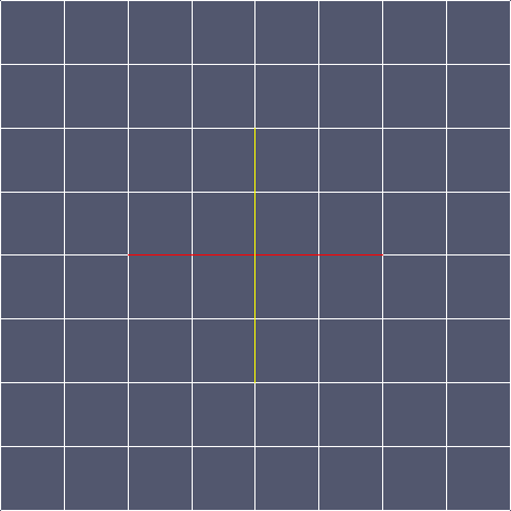
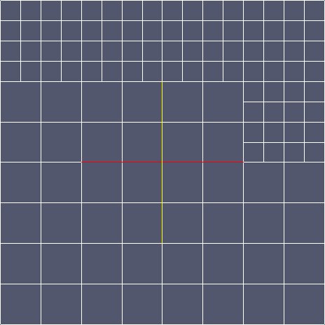
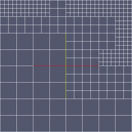
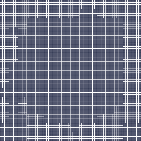
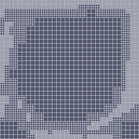
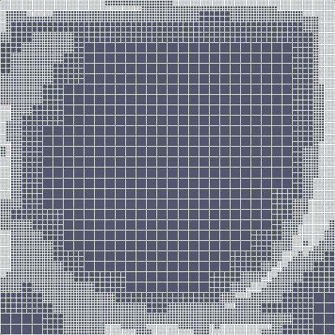
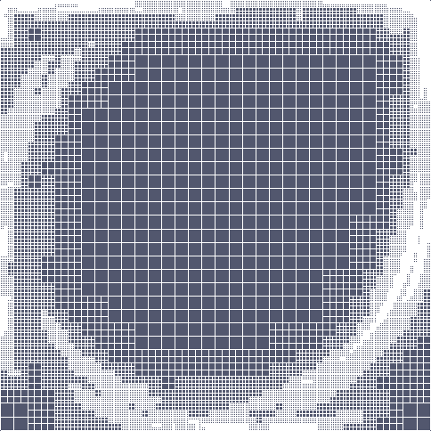
The following figures show the sequence of generated grids. For the case of \mathrm{Re}=400, the initial guess is obtained by solving Stokes on an 8 \times 8 mesh, and the mesh is refined adaptively. Between meshes, the solution from the coarse mesh is interpolated to the fine mesh to be used as an initial guess.
This picture is the graphical streamline result of lid-driven cavity with \mathrm{Re}=400. 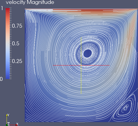
Then the solution is compared with a reference solution from [4] and the reference solution data can be found in the file "ref_2d_ghia_u.txt".

Test case 2: High Reynolds Number
Newton's iteration requires a good initial guess. However, the nonlinear term dominates when the Reynolds number is large, so that the solution to the Stokes equations may be far away from the exact solution. If the Stokes solution acts as the initial guess, the convergence will be lost. The following picture shows that the nonlinear iteration gets stuck and the residual no longer decreases in further iterations.

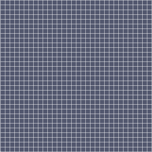
The initial guess, therefore, has to be obtained via a continuation method which has been discussed in the introduction. Here the step size in the continuation method, that is |\nu_{i}-\nu_{i+1}|, is 2000 and the initial mesh is of size 32 \times 32. After obtaining an initial guess, the mesh is refined as in the previous test case. The following picture shows that at each refinement Newton's iteration has quadratic convergence. 52 steps of Newton's iterations are executed for solving this test case.

We also show the residual from each step of Newton's iteration on every mesh. The quadratic convergence is clearly visible in the table.
| \mathrm{Re}=7500 | Mesh0 | Mesh1 | Mesh2 | Mesh3 | Mesh4 |
| Newton iter | Residual | FGMRES | Residual | FGMRES | Residual | FGMRES | Residual | FGMRES | Residual | FGMRES |
| 1 | 1.8922e-06 | 6 | 4.2506e-03 | 3 | 1.4299e-03 | 3 | 4.8793e-04 | 2 | 1.8998e-04 | 2 |
| 2 | 3.1644e-09 | 8 | 1.3732e-03 | 7 | 4.1506e-04 | 7 | 9.1119e-05 | 8 | 1.3555e-05 | 8 |
| 3 | 1.7611e-14 | 9 | 2.1946e-04 | 6 | 1.7881e-05 | 6 | 5.2678e-07 | 7 | 9.3739e-09 | 7 |
| 4 | | | 8.8269e-06 | 6 | 6.8210e-09 | 7 | 2.2770e-11 | 8 | 1.2588e-13 | 9 |
| 5 | | | 1.2974e-07 | 7 | 1.2515e-13 | 9 | 1.7801e-14 | 1 | | |
| 6 | | | 4.4352e-11 | 7 | | | | | | |
| 7 | | | 6.2863e-15 | 9 | | | | | | |
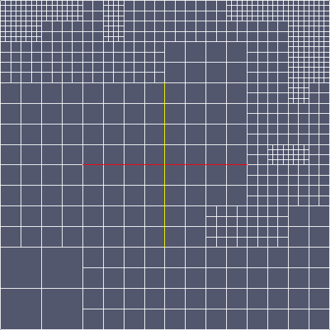
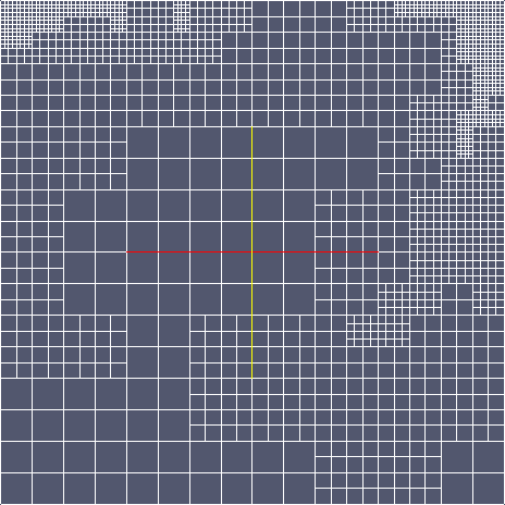
The sequence of generated grids looks like this:
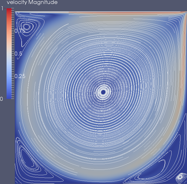
We compare our solution with reference solution from [5].  The following picture presents the graphical result.
Furthermore, the error consists of the nonlinear error, which decreases as we perform Newton iterations, and the discretization error, which depends on the mesh size. That is why we have to refine the mesh and repeat Newton's iteration on the next finer mesh. From the table above, we can see that the residual (nonlinear error) is below 1e-12 on each mesh, but the following picture shows us the difference between solutions on subsequently finer meshes.

Possibilities for extensions
Compare to other solvers
It is easy to compare the currently implemented linear solver to just using UMFPACK for the whole linear system. You need to remove the nullspace containing the constant pressures and it is done in step-56. More interesting is the comparison to other state of the art preconditioners like PCD. It turns out that the preconditioner here is very competitive, as can be seen in the paper [2].
The following table shows the timing results between our iterative approach (FGMRES) compared to a direct solver (UMFPACK) for the whole system with viscosity set to 1/400. Even though we use the same direct solver for the velocity block in the iterative solver, it is considerably faster and consumes less memory. This will be even more pronounced in 3d.
| Refinement Cycle | DoFs | Iterative: Total/s (Setup/s) | Direct: Total/s (Setup/s) |
| 5 | 9539 | 0.10 (0.06) | 0.13 (0.12) |
| 6 | 37507 | 0.58 (0.37) | 1.03 (0.97) |
| 7 | 148739 | 3.59 (2.73) | 7.78 (7.53) |
| 8 | 592387 | 29.17 (24.94) | (>4GB RAM) |
3d computations
The code is set up to also run in 3d. Of course the reference values are different, see [6] for example. High resolution computations are not doable with this example as is, because a direct solver for the velocity block does not work well in 3d. Rather, a parallel solver based on algebraic or geometric multigrid is needed. See below.
Parallelization
For larger computations, especially in 3d, it is necessary to implement MPI parallel solvers and preconditioners. A good starting point would be step-55, which uses algebraic multigrid for the velocity block for the Stokes equations. Another option would be to take a look at the list of codes in the deal.II code gallery, which already contains parallel Navier-Stokes solvers.
The plain program
#include <fstream>
#include <iostream>
namespace Step57
{
template <int dim>
class StationaryNavierStokes
{
public:
StationaryNavierStokes(const unsigned int degree);
void run(
const unsigned int refinement);
private:
void setup_dofs();
void initialize_system();
void assemble(
const bool initial_step,
const bool assemble_matrix);
void assemble_system(const bool initial_step);
void assemble_rhs(const bool initial_step);
void solve(const bool initial_step);
void refine_mesh();
void process_solution(unsigned int refinement);
void output_results(const unsigned int refinement_cycle) const;
void newton_iteration(const double tolerance,
const unsigned int max_n_line_searches,
const unsigned int max_n_refinements,
const bool is_initial_step,
const bool output_result);
void compute_initial_guess(double step_size);
double viscosity;
const unsigned int degree;
std::vector<types::global_dof_index> dofs_per_block;
};
template <int dim>
class BoundaryValues :
public Function<dim>
{
public:
BoundaryValues()
{}
const unsigned int component) const override;
};
template <int dim>
double BoundaryValues<dim>::value(
const Point<dim> & p,
const unsigned int component) const
{
Assert(component < this->n_components,
if (component == 0 &&
std::abs(p[dim - 1] - 1.0) < 1
e-10)
return 1.0;
return 0;
}
template <class PreconditionerMp>
{
public:
BlockSchurPreconditioner(
double gamma,
double viscosity,
const PreconditionerMp & Mppreconditioner);
private:
const double viscosity;
const PreconditionerMp & mp_preconditioner;
};
template <class PreconditionerMp>
BlockSchurPreconditioner<PreconditionerMp>::BlockSchurPreconditioner(
double viscosity,
const PreconditionerMp & Mppreconditioner)
, viscosity(viscosity)
, stokes_matrix(S)
, pressure_mass_matrix(P)
, mp_preconditioner(Mppreconditioner)
{
A_inverse.initialize(stokes_matrix.block(0, 0));
}
template <class PreconditionerMp>
void BlockSchurPreconditioner<PreconditionerMp>::vmult(
{
{
cg.solve(pressure_mass_matrix,
mp_preconditioner);
}
{
stokes_matrix.block(0, 1).vmult(utmp, dst.
block(1));
utmp *= -1.0;
}
A_inverse.vmult(dst.
block(0), utmp);
}
template <int dim>
StationaryNavierStokes<dim>::StationaryNavierStokes(const unsigned int degree)
: viscosity(1.0 / 7500.0)
, degree(degree)
, fe(
FE_Q<dim>(degree + 1), dim,
FE_Q<dim>(degree), 1)
{}
template <int dim>
void StationaryNavierStokes<dim>::setup_dofs()
{
system_matrix.clear();
pressure_mass_matrix.clear();
dof_handler.distribute_dofs(fe);
std::vector<unsigned int> block_component(dim + 1, 0);
block_component[dim] = 1;
dofs_per_block =
unsigned int dof_u = dofs_per_block[0];
unsigned int dof_p = dofs_per_block[1];
{
nonzero_constraints.clear();
0,
BoundaryValues<dim>(),
nonzero_constraints,
fe.component_mask(velocities));
}
nonzero_constraints.close();
{
zero_constraints.clear();
0,
dim + 1),
zero_constraints,
fe.component_mask(velocities));
}
zero_constraints.close();
std::cout <<
"Number of active cells: " <<
triangulation.n_active_cells()
<< std::endl
<< "Number of degrees of freedom: " << dof_handler.n_dofs()
<< " (" << dof_u << " + " << dof_p << ')' << std::endl;
}
template <int dim>
void StationaryNavierStokes<dim>::initialize_system()
{
{
sparsity_pattern.copy_from(dsp);
}
system_matrix.reinit(sparsity_pattern);
present_solution.reinit(dofs_per_block);
newton_update.reinit(dofs_per_block);
system_rhs.reinit(dofs_per_block);
}
template <int dim>
const bool assemble_matrix)
{
if (assemble_matrix)
system_matrix = 0;
system_rhs = 0;
quadrature_formula,
const unsigned int dofs_per_cell = fe.n_dofs_per_cell();
const unsigned int n_q_points = quadrature_formula.size();
std::vector<types::global_dof_index> local_dof_indices(dofs_per_cell);
std::vector<Tensor<1, dim>> present_velocity_values(n_q_points);
std::vector<Tensor<2, dim>> present_velocity_gradients(n_q_points);
std::vector<double> present_pressure_values(n_q_points);
std::vector<double> div_phi_u(dofs_per_cell);
std::vector<Tensor<1, dim>> phi_u(dofs_per_cell);
std::vector<Tensor<2, dim>> grad_phi_u(dofs_per_cell);
std::vector<double> phi_p(dofs_per_cell);
for (const auto &cell : dof_handler.active_cell_iterators())
{
fe_values.reinit(cell);
local_matrix = 0;
local_rhs = 0;
fe_values[velocities].get_function_values(evaluation_point,
present_velocity_values);
fe_values[velocities].get_function_gradients(
evaluation_point, present_velocity_gradients);
fe_values[pressure].get_function_values(evaluation_point,
present_pressure_values);
for (unsigned int q = 0; q < n_q_points; ++q)
{
for (unsigned int k = 0; k < dofs_per_cell; ++k)
{
div_phi_u[k] = fe_values[velocities].divergence(k, q);
grad_phi_u[k] = fe_values[velocities].gradient(k, q);
phi_u[k] = fe_values[velocities].value(k, q);
phi_p[k] = fe_values[pressure].value(k, q);
}
for (unsigned int i = 0; i < dofs_per_cell; ++i)
{
if (assemble_matrix)
{
for (unsigned int j = 0; j < dofs_per_cell; ++j)
{
local_matrix(i, j) +=
(viscosity *
present_velocity_gradients[q] * phi_u[j] * phi_u[i] +
grad_phi_u[j] * present_velocity_values[q] *
phi_u[i] -
div_phi_u[i] * phi_p[j] - phi_p[i] * div_phi_u[j] +
gamma * div_phi_u[j] * div_phi_u[i] +
phi_p[i] * phi_p[j]) *
fe_values.JxW(q);
}
}
double present_velocity_divergence =
trace(present_velocity_gradients[q]);
local_rhs(i) +=
grad_phi_u[i]) -
present_velocity_gradients[q] * present_velocity_values[q] *
phi_u[i] +
present_pressure_values[q] * div_phi_u[i] +
present_velocity_divergence * phi_p[i] -
gamma * present_velocity_divergence * div_phi_u[i]) *
fe_values.JxW(q);
}
}
cell->get_dof_indices(local_dof_indices);
initial_step ? nonzero_constraints : zero_constraints;
if (assemble_matrix)
{
local_rhs,
local_dof_indices,
system_matrix,
system_rhs);
}
else
{
local_dof_indices,
system_rhs);
}
}
if (assemble_matrix)
{
pressure_mass_matrix.reinit(sparsity_pattern.block(1, 1));
pressure_mass_matrix.copy_from(system_matrix.block(1, 1));
system_matrix.block(1, 1) = 0;
}
}
template <int dim>
void StationaryNavierStokes<dim>::assemble_system(const bool initial_step)
{
}
template <int dim>
void StationaryNavierStokes<dim>::assemble_rhs(const bool initial_step)
{
}
template <int dim>
void StationaryNavierStokes<dim>::solve(const bool initial_step)
{
initial_step ? nonzero_constraints : zero_constraints;
1
e-4 * system_rhs.l2_norm(),
true);
pmass_preconditioner.
initialize(pressure_mass_matrix,
const BlockSchurPreconditioner<SparseILU<double>> preconditioner(
viscosity,
system_matrix,
pressure_mass_matrix,
pmass_preconditioner);
gmres.solve(system_matrix, newton_update, system_rhs, preconditioner);
std::cout << "FGMRES steps: " << solver_control.last_step() << std::endl;
}
template <int dim>
void StationaryNavierStokes<dim>::refine_mesh()
{
dof_handler,
present_solution,
estimated_error_per_cell,
fe.component_mask(velocity));
estimated_error_per_cell,
0.3,
0.0);
solution_transfer.prepare_for_coarsening_and_refinement(present_solution);
setup_dofs();
solution_transfer.interpolate(present_solution, tmp);
nonzero_constraints.distribute(tmp);
initialize_system();
present_solution = tmp;
}
template <int dim>
void StationaryNavierStokes<dim>::newton_iteration(
const double tolerance,
const unsigned int max_n_line_searches,
const unsigned int max_n_refinements,
const bool is_initial_step,
const bool output_result)
{
bool first_step = is_initial_step;
for (unsigned int refinement_n = 0; refinement_n < max_n_refinements + 1;
++refinement_n)
{
unsigned int line_search_n = 0;
double last_res = 1.0;
double current_res = 1.0;
std::cout << "grid refinements: " << refinement_n << std::endl
<< "viscosity: " << viscosity << std::endl;
while ((first_step || (current_res > tolerance)) &&
line_search_n < max_n_line_searches)
{
if (first_step)
{
setup_dofs();
initialize_system();
evaluation_point = present_solution;
assemble_system(first_step);
solve(first_step);
present_solution = newton_update;
nonzero_constraints.distribute(present_solution);
first_step = false;
evaluation_point = present_solution;
assemble_rhs(first_step);
current_res = system_rhs.l2_norm();
std::cout << "The residual of initial guess is " << current_res
<< std::endl;
last_res = current_res;
}
else
{
evaluation_point = present_solution;
assemble_system(first_step);
solve(first_step);
for (
double alpha = 1.0; alpha > 1
e-5; alpha *= 0.5)
{
evaluation_point = present_solution;
evaluation_point.add(alpha, newton_update);
nonzero_constraints.distribute(evaluation_point);
assemble_rhs(first_step);
current_res = system_rhs.l2_norm();
std::cout << " alpha: " << std::setw(10) << alpha
<< std::setw(0) << " residual: " << current_res
<< std::endl;
if (current_res < last_res)
break;
}
{
present_solution = evaluation_point;
std::cout << " number of line searches: " << line_search_n
<< " residual: " << current_res << std::endl;
last_res = current_res;
}
++line_search_n;
}
if (output_result)
{
output_results(max_n_line_searches * refinement_n +
line_search_n);
if (current_res <= tolerance)
process_solution(refinement_n);
}
}
if (refinement_n < max_n_refinements)
{
refine_mesh();
}
}
}
template <int dim>
void StationaryNavierStokes<dim>::compute_initial_guess(double step_size)
{
const double target_Re = 1.0 / viscosity;
bool is_initial_step = true;
for (double Re = 1000.0; Re < target_Re;
Re =
std::min(Re + step_size, target_Re))
{
viscosity = 1.0 / Re;
std::cout << "Searching for initial guess with Re = " << Re
<< std::endl;
newton_iteration(1
e-12, 50, 0, is_initial_step,
false);
is_initial_step = false;
}
}
template <int dim>
void StationaryNavierStokes<dim>::output_results(
const unsigned int output_index) const
{
std::vector<std::string> solution_names(dim, "velocity");
solution_names.emplace_back("pressure");
std::vector<DataComponentInterpretation::DataComponentInterpretation>
data_component_interpretation(
data_component_interpretation.push_back(
solution_names,
data_component_interpretation);
}
template <int dim>
void StationaryNavierStokes<dim>::process_solution(unsigned int refinement)
{
f << "# y u_x u_y" << std::endl;
p(0) = 0.5;
p(1) = 0.5;
f << std::scientific;
for (unsigned int i = 0; i <= 100; ++i)
{
p(dim - 1) = i / 100.0;
f << p(dim - 1);
for (int j = 0; j < dim; j++)
f << " " << tmp_vector(j);
f << std::endl;
}
}
template <int dim>
{
const double Re = 1.0 / viscosity;
if (Re > 1000.0)
{
std::cout << "Searching for initial guess ..." << std::endl;
const double step_size = 2000.0;
compute_initial_guess(step_size);
std::cout << "Found initial guess." << std::endl;
std::cout << "Computing solution with target Re = " << Re << std::endl;
viscosity = 1.0 / Re;
newton_iteration(1
e-12, 50, refinement,
false,
true);
}
else
{
newton_iteration(1
e-12, 50, refinement,
true,
true);
}
}
}
int main()
{
try
{
using namespace Step57;
StationaryNavierStokes<2> flow( 1);
flow.run(4);
}
catch (std::exception &exc)
{
std::cerr << std::endl
<< std::endl
<< "----------------------------------------------------"
<< std::endl;
std::cerr << "Exception on processing: " << std::endl
<< exc.what() << std::endl
<< "Aborting!" << std::endl
<< "----------------------------------------------------"
<< std::endl;
return 1;
}
catch (...)
{
std::cerr << std::endl
<< std::endl
<< "----------------------------------------------------"
<< std::endl;
std::cerr << "Unknown exception!" << std::endl
<< "Aborting!" << std::endl
<< "----------------------------------------------------"
<< std::endl;
return 1;
}
return 0;
}



The following picture presents the graphical result.
