 |
Reference documentation for deal.II version 9.1.1
|
 |
Reference documentation for deal.II version 9.1.1
|
A module discussing the use of parallelism on distributed memory clusters. More...
Namespaces | |
| parallel::distributed | |
A module discussing the use of parallelism on distributed memory clusters.
deal.II can use multiple machine connected via MPI to parallelize computations, in addition to the parallelization within a shared memory machine discussed in the Parallel computing with multiple processors accessing shared memory module. There are essentially two ways to utilize multiple machines:
The first of these two options is relatively straightforward because most of the things one wants to do in a finite element program still work in essentially the same way, and handling distributed matrices, vectors, and linear solvers is something for which good external libraries such as Trilinos or PETSc exist that can make things look almost exactly the same as they would if everything was available locally. The use of this mode of parallelization is explained in the tutorial programs step-17, and step-18 and will not be discussed here in more detail.
The use of truly distributed meshes is somewhat more complex because it changes or makes impossible some of the things that can otherwise be done with deal.II triangulations, DoF handlers, etc. This module documents these issues with a vantage point at 50,000 ft above ground without going into too many details. All the algorithms described below are implement in classes and functions in namespace parallel::distributed.
One important aspect in parallel computations using MPI is that write access to matrix and vector elements requires a call to compress() after the operation is finished and before the object is used (for example read from). Also see GlossCompress.
A complete discussion of the algorithms used in this namespace, as well as a thorough description of many of the terms used here, can be found in the Distributed Computing paper. In particular, the paper shows that the methods discussed in this module scale to thousands of processors and well over a billion degrees of freedom (they may scale to even bigger problems but at the time of writing this, we do not have solvers that are capable of more than 2^{31} degrees of freedom due to the use of signed int as index). The paper also gives a concise definition of many of the terms that are used here and in other places of the library related to distributed computing. The step-40 tutorial program shows an application of the classes and methods of this namespace to the Laplace equation, while step-55 does so for a vector-valued problem. step-32 extends the step-31 program to massively parallel computations and thereby explains the use of the topic discussed here to more complicated applications.
For a discussion of what we consider "scalable" programs, see this glossary entry.
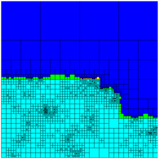
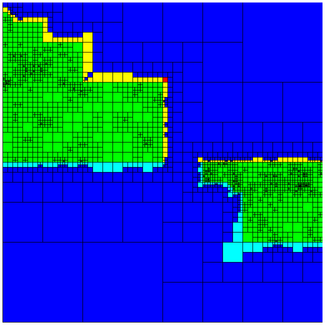
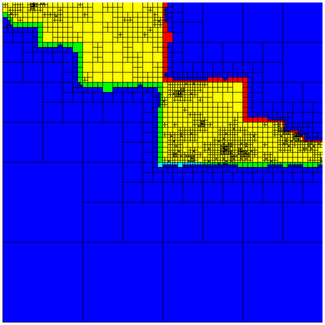
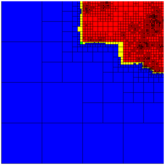
In parallel distributed mode, objects of type parallel::distributed::Triangulation on each processor only store a subset of cells. In particular, the global mesh can be thought of as decomposed so that each MPI process "owns" a number of cells. The mesh each process then stores locally consists of exactly those cells that it owns, as well as one layer of ghost cells around the ones it locally owns, and a number of cells we call artificial. The latter are cells that ensure that each processor has a mesh that has all the coarse level cells and that respects the invariant that neighboring cells can not differ by more than one level of refinement. The following pictures show such a mesh, distributed across four processors, and the collection of cells each of these processors stores locally:

| 
|

| 
|
The cells are colored based on the subdomain id, which identifies which processor owns a cell: turquoise for processor 0, green for processor 1, yellow for processor 2, and red for processor 3. As can be seen, each process has one layer of ghost cells around its own cells, which are correctly colored by the subdomain id that identifies the processor that owns each of these cells. Note also how each processor stores a number of artificial cells, indicated in blue, that only exist to ensure that each processor knows about all coarse grid cells and that the meshes have the 2:1 refinement property; however, in the area occupied by these artificial cells, a processor has no knowledge how refined the mesh there really is, as these are areas that are owned by other processors. As a consequence, all algorithms we will develop can only run over the locally owned cells and if necessary the ghost cells; trying to access data on any of the artificial cells is most likely an error. Note that we can determine whether we own a cell by testing that cell->subdomain_id() == triangulation.locally_owned_subdomain().
The "real" mesh one has to think of here is the one that would result from forming the union of cells each of the processes own, i.e. from the overlap of the turquoise, green, yellow and red areas, disregarding the blue areas.
The DoFHandler class builds on the Triangulation class, but it can detect whenever we actually use an object of type parallel::distributed::Triangulation as triangulation. In that case, it assigns global numbers for all degrees of freedom that exist, given a finite element, on the global mesh, but each processor will only know about those that are defined on locally relevant cells (i.e. cells either locally owned or that are ghost cells). Internally, the algorithm essentially works by just looping over all cells we own locally and assigning DoF indices to the degrees of freedom defined on them and, in the case of degrees of freedom at the interface between subdomains owned by different processors, that are not owned by the neighboring processor. All processors then exchange how many degrees of freedom they locally own and shift their own indices in such a way that every degree of freedom on all subdomains are uniquely identified by an index between zero and DoFHandler::n_dofs() (this function returns the global number of degrees of freedom, accumulated over all processors). Note that after this step, the degrees of freedom owned by each process form a contiguous range that can, for example, be obtained by the contiguous index set returned by DoFHandler::locally_owned_dofs(). After assigning unique indices to all degrees of freedom, the DoFHandler::distribute_dofs() function then loops over all ghost cells and communicates with neighboring processors to ensure that the global indices of degrees of freedom on these ghost cells match the ones that the neighbor has assigned to them.
Through this scheme, we can make sure that each cell we locally own as well as all the ghost cells can be asked to yield the globally correct indices for the degrees of freedom defined on them. However, asking for degrees of freedom on artificial cells is likely going to lead to nothing good, as no information is available for these cells (in fact, it isn't even known whether these cells are active on the global mesh, or are further refined).
As usual, degrees of freedom can be renumbered after being enumerated, using the functions in namespace DoFRenumbering.
One thing one learns very quickly when working with very large numbers of processors is that one can not store information about every degree of freedom on each processor, even if this information is "this degree of freedom doesn't live here". An example for this is that we can create an object for a (compressed) sparsity pattern that has DoFHandler::n_dofs() rows, but for which we fill only those rows that correspond to the DoFHandler::n_locally_owned_dofs() locally owned degrees of freedom. The reason is simple: for the sake of example, let's assume we have 1 billion degrees of freedom distributed across 100 processors; if we even only hold 16 bytes per line in this sparsity pattern (whether we own the corresponding DoF or not), we'll need 16 GB for this object even if every single line is empty. Of course, only 10 million lines will be non-empty, for which we need 160 MB plus whatever is necessary to store the actual column indices of nonzero entries. Let's say we have a moderately complex problem with 50 entries per row, for each of which we store the column index worth 4 bytes, then we'll need 216 bytes for each of the 10 million lines that correspond to the degrees of freedom we own, for a total of 2.16 GB. And we'll need 16 bytes for each of the 990 million lines that we don't own, for a total of 15.840 GB. It is clear that this ratio doesn't become any better if we go to even higher numbers of processors.
The solution to this problem is to really only use any memory at all for those parts of the linear system that we own, or need for some other reason. For all other parts, we must know that they exist, but we can not set up any part of our data structure. To this end, there exists a class called IndexSet that denotes a set of indices which we care for, and for which we may have to allocate memory. The data structures for sparsity patterns, constraint matrices, matrices and vector can be initialized with these IndexSet objects to really only care for those rows or entries that correspond to indices in the index set, and not care about all others. These objects will then ask how many indices exist in the set, allocate memory for each one of them (e.g. initialize the data structures for a line of a sparsity pattern), and when you want to access data for global degree of freedom i you will be redirected to the result of calling IndexSet::index_within_set() with index i instead. Accessing data for elements i for which IndexSet::is_element() is false will yield an error.
The remaining question is how to identify the set of indices that correspond to degrees of freedom we need to worry about on each processor. To this end, you can use the DoFTools::extract_locally_owned_dofs() function to get at all the indices a processor owns. Note that this is a subset of the degrees of freedom that are defined on the locally owned cells (since some of the degrees of freedom at the interface between two different subdomains may be owned by the neighbor). This set of degrees of freedom defined on cells we own can be obtained using the function DoFTools::extract_locally_active_dofs(). Finally, one sometimes needs the set of all degrees of freedom on the locally owned subdomain as well as the adjacent ghost cells. This information is provided by the DoFTools::extract_locally_relevant_dofs() function.
A typical parallel application is dealing with two different kinds of parallel vectors: vectors with ghost elements (also called ghosted vectors) and vectors without ghost elements. (Both kinds can typically be represented by the same data type, but there are of course different vector types that can each represent both flavors: for example TrilinosWrappers::MPI::Vector, PETScWrappers::MPI::Vector, and BlockVector objects built on these). You can find a discussion of what distinguishes these kinds of vectors in the glossary entry on ghosted vectors.
From a usage point of view, ghosted vectors are typically used for data output, postprocessing, error estimation, input in integration. This is because in these operations, one typically needs access not only to locally owned dofs but also to locally active dofs and sometimes to locally relevant dofs, and their values may not be stored in non-ghosted vectors on the processor that needs them. The operations listed above also only require read-only access to vectors, and ghosted vectors are therefore usable in these contexts.
On the other hand, vectors without ghost entries are used in all other places like assembling, solving, or any other form of manipulation. These are typically write-only operations and therefore need not have read access to vector elements that may be owned by another processor.
You can copy between vectors with and without ghost elements (you can see this in step-40, step-55, and step-32) using operator=.
At the time of writing this, the only class equipped to deal with the situation just explained is DynamicSparsityPattern. A version of the function DynamicSparsityPattern::reinit() exists that takes an IndexSet argument that indicates which lines of the sparsity pattern to allocate memory for. In other words, it is safe to create such an object that will report as its size 1 billion, but in fact only stores only as many rows as the index set has elements. You can then use the usual function DoFTools::make_sparsity_pattern to build the sparsity pattern that results from assembling on the locally owned portion of the mesh. The resulting object can be used to initialize a PETSc or Trilinos matrix which support very large object sizes through completely distributed storage. The matrix can then be assembled by only looping over those cells owned by the current processor.
The only thing to pay attention to is for which degrees of freedom the sparsity needs to store entries. These are, in essence, the ones we could possibly store values to in the matrix upon assembly. It is clear that these are certainly the locally active degrees of freedom (which live on the cells we locally own) but through constraints, it may also be possible to write to entries that are located on ghost cells. Consequently, you need to pass the index set that results from DoFTools::extract_locally_relevant_dofs() upon initializing the sparsity pattern.
When creating the sparsity pattern as well as when assembling the linear system, we need to know about constraints on degrees of freedom, for example resulting from hanging nodes or boundary conditions. Like the DynamicSparsityPattern class, the AffineConstraints container can also take an IndexSet upon construction that indicates for which of the possibly very large number of degrees of freedom it should actually store constraints. Unlike for the sparsity pattern, these are now only those degrees of freedom which we work on locally when assembling, namely those returned by DoFTools::extract_locally_active_dofs() (a superset of the locally owned ones).
There are, however, situations where more complicated constraints appear in finite element programs. An example is in hp adaptive computations where degrees of freedom can be constrained against other degrees of freedom that are themselves constrained. In a case like this, in order to fully resolve this chain of constraints, it may not be sufficient to only store constraints on locally active degrees of freedom but one may also need to have constraints available on locally relevant ones. In that case, the AffineConstraints object needs to be initialized with the IndexSet produced by DoFTools::extract_locally_relevant_dofs() .
In general, your program will continue to do something if you happen to not store all necessary constraints on each processor: you will just generate wrong matrix entries, but the program will not abort. This is opposed to the situation of the sparsity pattern: there, if the IndexSet passed to the DynamicSparsityPattern indicates that it should store too few rows of the matrix, the program will either abort when you attempt to write into matrix entries that do not exist or the matrix class will silently allocate more memory to accommodate them. As a consequence, it is useful to err on the side of caution when indicating which constraints to store and use the result of DoFTools::extract_locally_relevant_dofs() rather than DoFTools::extract_locally_active_dofs() . This is also affordable since the set of locally relevant degrees of freedom is only marginally larger than the set of locally active degrees of freedom. We choose this strategy in step-32, step-40, and step-55.
Like everything else, you can only do postprocessing on cells a local processor owns. The DataOut and KellyErrorEstimator classes do this automatically: they only operate on locally owned cells without the need to do anything in particular. At least for large computations, there is also no way to merge the results of all these local computations on a single machine, i.e. each processor has to be self-sufficient. For example, each processor has to generate its own parallel output files that have to be visualized by a program that can deal with multiple input files rather than merging the results of calling DataOut to a single processor before generating a single output file. The latter can be achieved, for example, using the DataOutBase::write_vtu() and DataOutBase::write_pvtu_record() functions.
These same considerations hold for all other postprocessing actions as well: while it is, for example, possible to compute a global energy dissipation rate by doing the computations locally and accumulating the resulting single number processor to a single number for the entire communication, it is in general not possible to do the same if the volume of data produced by every processor is significant.
There is one particular consideration for postprocessing, however: whatever you do on each cell a processor owns, you need access to at least all those values of the solution vector that are active on these cells (i.e. to the set of all locally active degrees of freedom, in the language of the Distributed Computing paper), which is a superset of the degrees of freedom this processor actually owns (because it may not own all degrees of freedom on the interface between its own cells and those cells owned by other processors). Sometimes, however, you need even more information: for example, to compute the KellyErrorIndicator results, one needs to evaluate the gradient at the interface on the current as well as its neighbor cell; the latter may be owned by another processor, so we need those degrees of freedom as well. In general, therefore, one needs access to the solution values for all degrees of freedom that are locally relevant. On the other hand, both of the packages we can use for parallel linear algebra (PETSc and Trilinos) as well as parallel::distributed::Vector subdivide vectors into chunks each processor owns and chunks stored on other processors. To postprocess stuff therefore means that we have to tell PETSc or Trilinos that it should also import ghost elements, i.e. additional vector elements of the solution vector other than the ones we own locally. For ghosted vectors, this can be achieved by using operator= with a distributed vector as argument.
 1.8.14