 |
Reference documentation for deal.II version 9.6.0
|
 |
Reference documentation for deal.II version 9.6.0
|
This tutorial depends on step-6.
| Table of contents | |
|---|---|
This program was contributed by Timo Heister, Martin Kronbichler, and Wolfgang Bangerth.
This material is based upon work partly supported by the National Science Foundation under Award No. EAR-0426271 and The California Institute of Technology. Any opinions, findings, and conclusions or recommendations expressed in this publication are those of the author and do not necessarily reflect the views of the National Science Foundation or of The California Institute of Technology.
Given today's computers, many finite element computations can be done on a single machine. The majority of previous tutorial programs therefore shows only this, possibly splitting up work among a number of processors that, however, can all access the same, shared memory space. That said, there are problems that are simply too big for a single machine and in that case the problem has to be split up in a suitable way among multiple machines each of which contributes its part to the whole. A simple way to do that was shown in step-17 and step-18, where we show how a program can use MPI to parallelize assembling the linear system, storing it, solving it, and computing error estimators. All of these operations scale relatively trivially (for a definition of what it means for an operation to "scale", see this glossary entry), but there was one significant drawback: For this to be moderately simple to implement, each MPI processor had to keep its own copy of the entire Triangulation and DoFHandler objects. Consequently, while we can suspect (with good reasons) that the operations listed above can scale to thousands of computers and problem sizes of billions of cells and billions of degrees of freedom, building the one big mesh for the entire problem these thousands of computers are solving on every last processor is clearly not going to scale: it is going to take forever, and maybe more importantly no single machine will have enough memory to store a mesh that has a billion cells (at least not at the time of writing this). In reality, programs like step-17 and step-18 can therefore not be run on more than maybe 100 or 200 processors, and even then storing the Triangulation and DoFHandler objects consumes the vast majority of memory on each machine.
Consequently, we need to approach the problem differently: to scale to very large problems, each processor can only store its own little piece of the Triangulation and DoFHandler objects. deal.II implements such a scheme in the parallel::distributed namespace and the classes therein. It builds on an external library, p4est (a word play on the expression parallel forest that describes the parallel storage of a hierarchically constructed mesh as a forest of quad- or oct-trees). You need to install p4est and configure deal.II to use it, but apart from that, all of its workings are hidden under the surface of deal.II.
In essence, what the parallel::distributed::Triangulation class and code inside the DoFHandler class do is to split the global mesh so that every processor only stores a small bit it "owns" along with one layer of "ghost" cells that surround the ones it owns. What happens in the rest of the domain on which we want to solve the partial differential equation is unknown to each processor and can only be inferred through communication with other machines if such information is needed. This implies that we also have to think about problems in a different way than we did in, for example, step-17 and step-18: no processor can have the entire solution vector for postprocessing, for example, and every part of a program has to be parallelized because no processor has all the information necessary for sequential operations.
A general overview of how this parallelization happens is described in the Parallel computing with multiple processors using distributed memory documentation topic. You should read it for a top-level overview before reading through the source code of this program. A concise discussion of many terms we will use in the program is also provided in the Distributed Computing paper. It is probably worthwhile reading it for background information on how things work internally in this program.
step-17 and step-18 already used parallel linear algebra classes, but since the current program is the first one that really covers parallel computing, it is probably worth giving a broad overview of parallel linear algebra here as well.
First, the general mantra mentioned above was that everything has to be distributed. It does not scale if one process (or in fact all processes) have to keep a complete triangulation or even a substantial share of it; it all only works if every one of the N processes in the parallel universe keep at most a small multiple of one Nth of the triangulation. Similarly, each process can only hold a small multiple of one Nth of each solution or right hand side vector, and of the system matrix.
To this end, deal.II has acquired interfaces to a number of packages that provide these kind of distributed linear algebra data structures. More specifically, deal.II comes with a number of "sub-packages" that all provide vector, matrix, and linear solver classes that are typically named the same or very similarly, but live in different namespaces:
namespace dealii.PETScWrappers. PETSc is a library that has built a large collection of linear algebra, linear solvers, nonlinear solvers, time steppers, and other functionality that runs on some of the largest machines in the world in parallel, using MPI.For the current program, we need to use parallel linear algebra classes to represent the matrix and vectors. Both the PETScWrapper and TrilinosWrapper classes will fit the bill and, depending on whether deal.II was configured with one or the other (or both), the top of the program selects one or the other set of wrappers by putting the respective class names into a namespace LA.
This program essentially re-solves what we already do in step-6, i.e. it solves the Laplace equation
\begin{align*} -\Delta u &= f \qquad &&\text{in}\ \Omega=[0,1]^2, \\ u &= 0 \qquad &&\text{on}\ \partial\Omega. \end{align*}
The difference of course is now that we want to do so on a mesh that may have a billion cells, with a billion or so degrees of freedom. There is no doubt that doing so is completely silly for such a simple problem, but the point of a tutorial program is, after all, not to do something useful but to show how useful programs can be implemented using deal.II. Be that as it may, to make things at least a tiny bit interesting, we choose the right hand side as a discontinuous function,
\begin{align*} f(x,y) = \left\{ \begin{array}{ll} 1 & \text{if}\ y > \frac 12 + \frac 14 \sin(4\pi x), \\ -1 & \text{otherwise}, \end{array} \right. \end{align*}
so that the solution has a singularity along the sinusoidal line snaking its way through the domain. As a consequence, mesh refinement will be concentrated along this line. You can see this in the mesh picture shown below in the results section.
Rather than continuing here and giving a long introduction, let us go straight to the program code. If you have read through step-6 and the Parallel computing with multiple processors using distributed memory documentation topic, most of things that are going to happen should be familiar to you already. In fact, comparing the two programs you will notice that the additional effort necessary to make things work in parallel is almost insignificant: the two programs have about the same number of lines of code (though step-6 spends more space on dealing with coefficients and output). In either case, the comments below will only be on the things that set step-40 apart from step-6 and that aren't already covered in the Parallel computing with multiple processors using distributed memory documentation topic.
unsigned int, which on most machines today is a 32-bit integer, limiting you to some 4 billion (in reality, since this program uses PETSc, you will be limited to half that as PETSc uses signed integers). However, this can be changed during configuration to use 64-bit integers, see the ReadMe file. This will give problem sizes you are unlikely to exceed anytime soon.Most of the include files we need for this program have already been discussed in previous programs. In particular, all of the following should already be familiar friends:
This program can use either PETSc or Trilinos for its parallel algebra needs. By default, if deal.II has been configured with PETSc, it will use PETSc. Otherwise, the following few lines will check that deal.II has been configured with Trilinos and take that.
But there may be cases where you want to use Trilinos, even though deal.II has also been configured with PETSc, for example to compare the performance of these two libraries. To do this, add the following #define to the source code:
Using this logic, the following lines will then import either the PETSc or Trilinos wrappers into the namespace LA (for linear algebra). In the former case, we are also defining the macro USE_PETSC_LA so that we can detect if we are using PETSc (see solve() for an example where this is necessary).
The following, however, will be new or be used in new roles. Let's walk through them. The first of these will provide the tools of the Utilities::System namespace that we will use to query things like the number of processors associated with the current MPI universe, or the number within this universe the processor this job runs on is:
The next one provides a class, ConditionOStream that allows us to write code that would output things to a stream (such as std::cout) on every processor but throws the text away on all but one of them. We could achieve the same by simply putting an if statement in front of each place where we may generate output, but this doesn't make the code any prettier. In addition, the condition whether this processor should or should not produce output to the screen is the same every time – and consequently it should be simple enough to put it into the statements that generate output itself.
After these preliminaries, here is where it becomes more interesting. As mentioned in the Parallel computing with multiple processors using distributed memory topic, one of the fundamental truths of solving problems on large numbers of processors is that there is no way for any processor to store everything (e.g. information about all cells in the mesh, all degrees of freedom, or the values of all elements of the solution vector). Rather, every processor will own a few of each of these and, if necessary, may know about a few more, for example the ones that are located on cells adjacent to the ones this processor owns itself. We typically call the latter ghost cells, ghost nodes or ghost elements of a vector. The point of this discussion here is that we need to have a way to indicate which elements a particular processor owns or need to know of. This is the realm of the IndexSet class: if there are a total of N cells, degrees of freedom, or vector elements, associated with (non-negative) integral indices [0,N), then both the set of elements the current processor owns as well as the (possibly larger) set of indices it needs to know about are subsets of the set [0,N). IndexSet is a class that stores subsets of this set in an efficient format:
The next header file is necessary for a single function, SparsityTools::distribute_sparsity_pattern. The role of this function will be explained below.
The final two, new header files provide the class parallel::distributed::Triangulation that provides meshes distributed across a potentially very large number of processors, while the second provides the namespace parallel::distributed::GridRefinement that offers functions that can adaptively refine such distributed meshes:
LaplaceProblem class templateNext let's declare the main class of this program. Its structure is almost exactly that of the step-6 tutorial program. The only significant differences are:
mpi_communicator variable that describes the set of processors we want this code to run on. In practice, this will be MPI_COMM_WORLD, i.e. all processors the batch scheduling system has assigned to this particular job.pcout variable of type ConditionOStream.LaplaceProblem class implementationConstructors and destructors are rather trivial. In addition to what we do in step-6, we set the set of processors we want to work on to all machines available (MPI_COMM_WORLD); ask the triangulation to ensure that the mesh remains smooth and free to refined islands, for example; and initialize the pcout variable to only allow processor zero to output anything. The final piece is to initialize a timer that we use to determine how much compute time the different parts of the program take:
The following function is, arguably, the most interesting one in the entire program since it goes to the heart of what distinguishes parallel step-40 from sequential step-6.
At the top we do what we always do: tell the DoFHandler object to distribute degrees of freedom. Since the triangulation we use here is distributed, the DoFHandler object is smart enough to recognize that on each processor it can only distribute degrees of freedom on cells it owns; this is followed by an exchange step in which processors tell each other about degrees of freedom on ghost cell. The result is a DoFHandler that knows about the degrees of freedom on locally owned cells and ghost cells (i.e. cells adjacent to locally owned cells) but nothing about cells that are further away, consistent with the basic philosophy of distributed computing that no processor can know everything.
The next two lines extract some information we will need later on, namely two index sets that provide information about which degrees of freedom are owned by the current processor (this information will be used to initialize solution and right hand side vectors, and the system matrix, indicating which elements to store on the current processor and which to expect to be stored somewhere else); and an index set that indicates which degrees of freedom are locally relevant (i.e. live on cells that the current processor owns or on the layer of ghost cells around the locally owned cells; we need all of these degrees of freedom, for example, to estimate the error on the local cells).
Next, let us initialize the solution and right hand side vectors. As mentioned above, the solution vector we seek does not only store elements we own, but also ghost entries; on the other hand, the right hand side vector only needs to have the entries the current processor owns since all we will ever do is write into it, never read from it on locally owned cells (of course the linear solvers will read from it, but they do not care about the geometric location of degrees of freedom).
The next step is to compute hanging node and boundary value constraints, which we combine into a single object storing all constraints.
As with all other things in parallel, the mantra must be that no processor can store all information about the entire universe. As a consequence, we need to tell the AffineConstraints object for which degrees of freedom it can store constraints and for which it may not expect any information to store. In our case, as explained in the Parallel computing with multiple processors using distributed memory topic, the degrees of freedom we need to care about on each processor are the locally relevant ones, so we pass this to the AffineConstraints::reinit() function as a second argument. A further optimization, AffineConstraint can avoid certain operations if you also provide it with the set of locally owned degrees of freedom – the first argument to AffineConstraints::reinit().
(What would happen if we didn't pass this information to AffineConstraints, for example if we called the argument-less version of AffineConstraints::reinit() typically used in non-parallel codes? In that case, the AffineConstraints class will allocate an array with length equal to the largest DoF index it has seen so far. For processors with large numbers of MPI processes, this may be very large – maybe on the order of billions. The program would then allocate more memory than for likely all other operations combined for this single array. Fortunately, recent versions of deal.II would trigger an assertion that tells you that this is considered a bug.)
The last part of this function deals with initializing the matrix with accompanying sparsity pattern. As in previous tutorial programs, we use the DynamicSparsityPattern as an intermediate with which we then initialize the system matrix. To do so, we have to tell the sparsity pattern its size, but as above, there is no way the resulting object will be able to store even a single pointer for each global degree of freedom; the best we can hope for is that it stores information about each locally relevant degree of freedom, i.e., all those that we may ever touch in the process of assembling the matrix (the distributed computing paper has a long discussion why one really needs the locally relevant, and not the small set of locally active degrees of freedom in this context).
So we tell the sparsity pattern its size and what DoFs to store anything for and then ask DoFTools::make_sparsity_pattern to fill it (this function ignores all cells that are not locally owned, mimicking what we will do below in the assembly process). After this, we call a function that exchanges entries in these sparsity pattern between processors so that in the end each processor really knows about all the entries that will exist in that part of the finite element matrix that it will own. The final step is to initialize the matrix with the sparsity pattern.
The function that then assembles the linear system is comparatively boring, being almost exactly what we've seen before. The points to watch out for are:
cell->subdomain_id() == triangulation.locally_owned_subdomain(), or skip all cells for which the condition cell->is_ghost() || cell->is_artificial() is true. The simplest way, however, is to simply ask the cell whether it is owned by the local processor.compress() function on the global matrix and right hand side vector objects (see the description of what this does just before these calls).In the operations above, specifically the call to distribute_local_to_global() in the last line, every MPI process was only working on its local data. If the operation required adding something to a matrix or vector entry that is not actually stored on the current process, then the matrix or vector object keeps track of this for a later data exchange, but for efficiency reasons, this part of the operation is only queued up, rather than executed right away. But now that we got here, it is time to send these queued-up additions to those processes that actually own these matrix or vector entries. In other words, we want to "finalize" the global data structures. This is done by invoking the function compress() on both the matrix and vector objects. See Compressing distributed objects for more information on what compress() actually does.
Even though solving linear systems on potentially tens of thousands of processors is by far not a trivial job, the function that does this is – at least at the outside – relatively simple. Most of the parts you've seen before. There are really only two things worth mentioning:
The function that estimates the error and refines the grid is again almost exactly like the one in step-6. The only difference is that the function that flags cells to be refined is now in namespace parallel::distributed::GridRefinement – a namespace that has functions that can communicate between all involved processors and determine global thresholds to use in deciding which cells to refine and which to coarsen.
Note that we didn't have to do anything special about the KellyErrorEstimator class: we just give it a vector with as many elements as the local triangulation has cells (locally owned cells, ghost cells, and artificial ones), but it only fills those entries that correspond to cells that are locally owned.
Compared to the corresponding function in step-6, the one here is a tad more complicated. There are two reasons: the first one is that we do not just want to output the solution but also for each cell which processor owns it (i.e. which "subdomain" it is in). Secondly, as discussed at length in step-17 and step-18, generating graphical data can be a bottleneck in parallelizing. In those two programs, we simply generate one output file per process. That worked because the parallel::shared::Triangulation cannot be used with large numbers of MPI processes anyway. But this doesn't scale: Creating a single file per processor will overwhelm the filesystem with a large number of processors.
We here follow a more sophisticated approach that uses high-performance, parallel IO routines using MPI I/O to write to a small, fixed number of visualization files (here 8). We also generate a .pvtu record referencing these .vtu files, which can be opened directly in visualizatin tools like ParaView and VisIt.
To start, the top of the function looks like it usually does. In addition to attaching the solution vector (the one that has entries for all locally relevant, not only the locally owned, elements), we attach a data vector that stores, for each cell, the subdomain the cell belongs to. This is slightly tricky, because of course not every processor knows about every cell. The vector we attach therefore has an entry for every cell that the current processor has in its mesh (locally owned ones, ghost cells, and artificial cells), but the DataOut class will ignore all entries that correspond to cells that are not owned by the current processor. As a consequence, it doesn't actually matter what values we write into these vector entries: we simply fill the entire vector with the number of the current MPI process (i.e. the subdomain_id of the current process); this correctly sets the values we care for, i.e. the entries that correspond to locally owned cells, while providing the wrong value for all other elements – but these are then ignored anyway.
The final step is to write this data to disk. We write up to 8 VTU files in parallel with the help of MPI-IO. Additionally a PVTU record is generated, which groups the written VTU files.
The function that controls the overall behavior of the program is again like the one in step-6. The minor difference are the use of pcout instead of std::cout for output to the console (see also step-17).
A functional difference to step-6 is the use of a square domain and that we start with a slightly finer mesh (5 global refinement cycles) – there just isn't much of a point showing a massively parallel program starting on 4 cells (although admittedly the point is only slightly stronger starting on 1024).
The final function, main(), again has the same structure as in all other programs, in particular step-6. Like the other programs that use MPI, we have to initialize and finalize MPI, which is done using the helper object Utilities::MPI::MPI_InitFinalize. The constructor of that class also initializes libraries that depend on MPI, such as p4est, PETSc, SLEPc, and Zoltan (though the last two are not used in this tutorial). The order here is important: we cannot use any of these libraries until they are initialized, so it does not make sense to do anything before creating an instance of Utilities::MPI::MPI_InitFinalize.
After the solver finishes, the LaplaceProblem destructor will run followed by Utilities::MPI::MPI_InitFinalize::~MPI_InitFinalize(). This order is also important: Utilities::MPI::MPI_InitFinalize::~MPI_InitFinalize() calls PetscFinalize (and finalization functions for other libraries), which will delete any in-use PETSc objects. This must be done after we destruct the Laplace solver to avoid double deletion errors. Fortunately, due to the order of destructor call rules of C++, we do not need to worry about any of this: everything happens in the correct order (i.e., the reverse of the order of construction). The last function called by Utilities::MPI::MPI_InitFinalize::~MPI_InitFinalize() is MPI_Finalize: i.e., once this object is destructed the program should exit since MPI will no longer be available.
When you run the program, on a single processor or with your local MPI installation on a few, you should get output like this:
The exact numbers differ, depending on how many processors we use; this is due to the fact that the preconditioner depends on the partitioning of the problem, the solution then differs in the last few digits, and consequently the mesh refinement differs slightly. The primary thing to notice here, though, is that the number of iterations does not increase with the size of the problem. This guarantees that we can efficiently solve even the largest problems.
When run on a sufficiently large number of machines (say a few thousand), this program can relatively easily solve problems with well over one billion unknowns in less than a minute. On the other hand, such big problems can no longer be visualized, so we also ran the program on only 16 processors. Here are a mesh, along with its partitioning onto the 16 processors, and the corresponding solution:
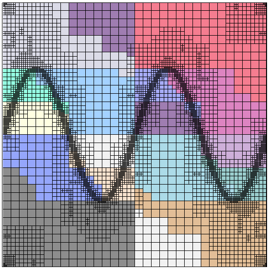 | 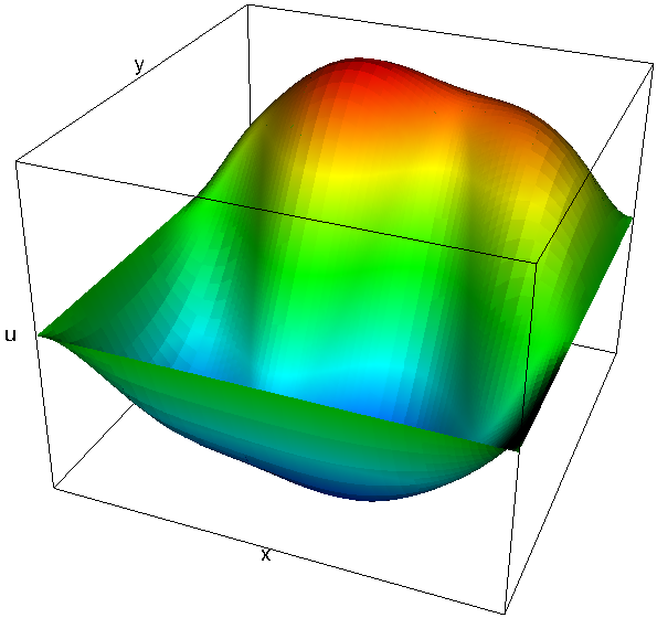 |
The mesh on the left has a mere 7,069 cells. This is of course a problem we would easily have been able to solve already on a single processor using step-6, but the point of the program was to show how to write a program that scales to many more machines. For example, here are two graphs that show how the run time of a large number of parts of the program scales on problems with around 52 and 375 million degrees of freedom if we take more and more processors (these and the next couple of graphs are taken from an earlier version of the Distributed Computing paper; updated graphs showing data of runs on even larger numbers of processors, and a lot more interpretation can be found in the final version of the paper):
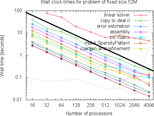 | 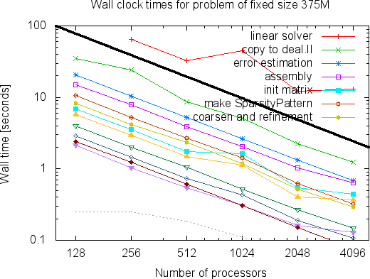 |
As can clearly be seen, the program scales nicely to very large numbers of processors. (For a discussion of what we consider "scalable" programs, see this glossary entry.) The curves, in particular the linear solver, become a bit wobbly at the right end of the graphs since each processor has too little to do to offset the cost of communication (the part of the whole problem each processor has to solve in the above two examples is only 13,000 and 90,000 degrees of freedom when 4,096 processors are used; a good rule of thumb is that parallel programs work well if each processor has at least 100,000 unknowns).
While the strong scaling graphs above show that we can solve a problem of fixed size faster and faster if we take more and more processors, the more interesting question may be how big problems can become so that they can still be solved within a reasonable time on a machine of a particular size. We show this in the following two graphs for 256 and 4096 processors:
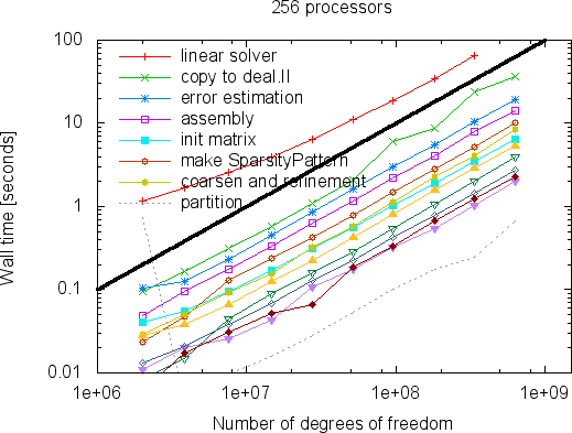 | 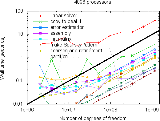 |
What these graphs show is that all parts of the program scale linearly with the number of degrees of freedom. This time, lines are wobbly at the left as the size of local problems is too small. For more discussions of these results we refer to the Distributed Computing paper.
So how large are the largest problems one can solve? At the time of writing this problem, the limiting factor is that the program uses the BoomerAMG algebraic multigrid method from the Hypre package as a preconditioner, which unfortunately uses signed 32-bit integers to index the elements of a distributed matrix. This limits the size of problems to 2^{31}-1=2,147,483,647 degrees of freedom. From the graphs above it is obvious that the scalability would extend beyond this number, and one could expect that given more than the 4,096 machines shown above would also further reduce the compute time. That said, one can certainly expect that this limit will eventually be lifted by the hypre developers.
On the other hand, this does not mean that deal.II cannot solve bigger problems. Indeed, step-37 shows how one can solve problems that are not just a little, but very substantially larger than anything we have shown here.
In a sense, this program is the ultimate solver for the Laplace equation: it can essentially solve the equation to whatever accuracy you want, if only you have enough processors available. Since the Laplace equation by itself is not terribly interesting at this level of accuracy, the more interesting possibilities for extension therefore concern not so much this program but what comes beyond it. For example, several of the other programs in this tutorial have significant run times, especially in 3d. It would therefore be interesting to use the techniques explained here to extend other programs to support parallel distributed computations. We have done this for step-31 in the step-32 tutorial program, but the same would apply to, for example, step-23 and step-25 for hyperbolic time dependent problems, step-33 for gas dynamics, or step-35 for the Navier-Stokes equations.
Maybe equally interesting is the problem of postprocessing. As mentioned above, we only show pictures of the solution and the mesh for 16 processors because 4,096 processors solving 1 billion unknowns would produce graphical output on the order of several 10 gigabyte. Currently, no program is able to visualize this amount of data in any reasonable way unless it also runs on at least several hundred processors. There are, however, approaches where visualization programs directly communicate with solvers on each processor with each visualization process rendering the part of the scene computed by the solver on this processor. Implementing such an interface would allow to quickly visualize things that are otherwise not amenable to graphical display.