 |
Reference documentation for deal.II version 9.4.1
|
 |
Reference documentation for deal.II version 9.4.1
|
This program was contributed by Joshua Christopher <chrisjoshtopher@gmail.com>.
It comes without any warranty or support by its authors or the authors of deal.II.
This program is part of the deal.II code gallery and consists of the following files (click to inspect):
 |  |
Over the last few years, the clock speed per processor core has stagnated. This stagnation has lead to the design of larger core counts in high performance computing machines. As a result of these developments, increased concurrency in numerical algorithms must be developed in order to take advantage of this architecture style. Perhaps the largest bottleneck in concurrency for time-dependent simulations is traditional time integration methods. Traditional time integration methods solve for the time domain sequentially, and as the spatial grid is refined a proportionally larger number of time steps must be taken to maintain accuracy and stability constraints. While solving the time domain sequentially with a traditional time integration method is an optimal algorithm of order \mathcal{O}(n), the n time steps are not solved concurrently.
The goal of this project is to make use of the XBraid library from Lawrence Livermore National Laboratory to solve the time domain in parallel using multigrid reduction in time techniques. The XBraid library is implemented in C and aims to be a non-intrusive method to implement parallel time marching methods into existing codes.
In order to use the XBraid library, several data structures and functions must be implemented and provided to the XBraid solver struct. The two required data structures are the app and vector structures. In general, the app struct contains the time independent data and the vector struct contains the time dependent data. For this initial example, the time independent data includes the mesh which is fixed for all time steps, and the time dependent data is the solution state vector. The functions tell XBraid how to perform operations on the data type used by your solver, in this case deal.II uses the Vector data type. These operations include how to initialize the data at a given time, how to sum the data, and how to pack and unpack linear buffers for transmission to other processors via MPI. The XBraid documentation should be read for a full list of functions that must be implemented and the details of what the function should do.
The typical format is the function is called with arguments of the app struct, one or more vector structs, and a status struct that contains information on the current status of the XBraid simulation (the current multigrid iteration, the level the function is being called from, the time and timestep number, etc.).
Perhaps the most important function is the step function. This function tells XBraid how to advance the solution forward in time from the initial to the final times given in the status struct. This method uses a traditional time integration method such as the fourth order explicit Runge Kutta method.
The solver used in this example is based off the heat equation solver from the step-26 tutorial of deal.II. The HeatEquation class becomes member data to XBraid’s app struct, and XBraid’s vector struct becomes a wrapper for deal.II’s Vector data type. The HeatEquation class cannot simply be used as is though as it contains both time dependent and time independent member data. In order to simplify the problem the adaptive mesh refinement is removed. Theoretically XBraid is capable of working with adaptive mesh refinement and in fact contains support for time refinement (which is also not used for simplicity). All adaptive mesh refinement functionality is removed from the solver. The time-dependent solution state vectors are also removed from the HeatEquation member data. That time-dependent data will be provided at each timestep by XBraid via the vector struct.
In the default mode, this code solves the heat equation,
\begin{align} \frac{\partial u}{\partial t} - \Delta u = f(\boldsymbol{x},t), \qquad \forall\boldsymbol{x}\in\Omega,t\in\left( 0,T \right), \end{align}
with initial conditions,
\begin{align} u(\boldsymbol{x},0) = u_0(\boldsymbol{x}) = 0, \qquad \forall \boldsymbol{x}\in\Omega, \end{align}
and Dirichlet boundary conditions,
\begin{align} u(\boldsymbol{x},t) = g(\boldsymbol{x},t) = 0, \qquad \forall \boldsymbol{x}\in\partial\Omega,t\in\left( 0,T \right) \end{align}
and forcing function,
\begin{align} f(\mathbf x, t) = \left\{ \begin{array}{ll} \chi_1(t) & \text{if \(x>0.5\) and \(y>-0.5\)} \\ \chi_2(t) & \text{if \(x>-0.5\) and \(y>0.5\)} \end{array} \right. \end{align}
with,
\begin{align} \chi_1(t) = \exp\left(-0.5\frac{(t-0.125)^2}{0.005}\right) \end{align}
and,
\begin{align} \chi_2(t) = \exp\left(-0.5\frac{(t-0.375)^2}{0.005}\right) \end{align}
for some time t. The forcing function is a Gaussian pulse in time that is centered around 0.125 time units for \chi_1 and 0.375 time units for \chi_2. A Gaussian function was chosen because it is a continuous function in time and so the solution state can be compared bit-wise with the serial-in-time solution.
The method of manufactured solutions is used to test the correctness of the implementation. In the method of manufactured solutions, we create a solution u_h to the heat equation, then compute the boundary conditions, initial conditions, and forcing functions required to generate that solution. This method is explained further in the step-7 tutorial of deal.II. The created solution used is,
\begin{align} u_h = \exp\left( -4\pi^2t \right) \cos(2 \pi x) \cos(2 \pi y), \qquad \forall \boldsymbol{x} \in \Omega \cup \partial\Omega \end{align}
with derivatives,
\begin{align} \frac{\partial u}{\partial t} &= -4 \pi^2 \exp{-4\pi 2t} \cos(2 \pi x)\cos(2 \pi y), \\ -\Delta u &= 8 \pi^2 \exp\left(-4\pi^2t\right)\cos(2 \pi x)\cos(2 \pi y) \\ \frac{\partial u}{\partial x} &= -2\pi \exp\left(-4\pi^2t\right)\sin(2\pi x)\cos(2\pi y) \\ \frac{\partial u}{\partial x} &= -2 \pi \exp\left(-4\pi^2t\right)\cos(2\pi x)\sin(2\pi y) \end{align}
and therefore we specify the forcing term, initial conditions, and boundary conditions of the governing equations as,
\begin{align} f(\boldsymbol{x},t) &= 4 \pi^2 \exp\left(-4\pi^2t\right)\cos(2 \pi x)\cos(2 \pi y), &&\forall\boldsymbol{x}\in\Omega,t\in\left( 0,T \right), \\ u_0(\boldsymbol{x}) &= \cos(2 \pi x)\cos(2\pi y), &&\forall \boldsymbol{x}\in\Omega, \\ g(\boldsymbol{x},t) &= \exp\left(-4\pi^2t\right)\cos(2 \pi x)\cos(2\pi y), &&\forall \boldsymbol{x} \in \partial\Omega. \end{align}
The manufactured solution is run on progressively more refined grids and the solution generated by the finite element method is compared to the exact solution u_h. The convergence rate of the error is calculated with
\begin{align} \Delta \epsilon_n = \frac{\ln{\epsilon_{n-1}/\epsilon_{n}}}{\ln{\frac\Delta x_{n-1}/\Delta x_{n}}} \end{align}
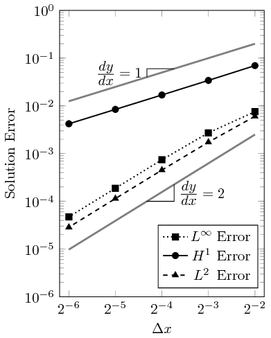
where \Delta \epsilon_n is the convergence rate of error \epsilon between a mesh n and coarser mesh n-1 that have a refinement ratio of r_n. Shown in Table 1 are the errors of the \textrm{L}^2, \textrm{H}^1, and \textrm{L}^\infty norms as the mesh is refined, and shown in Table 2 is the convergence rate. The \Delta t is reduced by a factor of 2 for every global refinement of the mesh.
\begin{align} \begin{tabular}{|c|c|c|c|c|c|} \hline cycles & \# cells & \# dofs & @f$\textrm{L}^2@f$-error & @f$\textrm{H}^1@f$-error & @f$\textrm{L}^\infty@f$-error \\ \hline 125 & 48 & 65 & 6.036e-03 & 6.970e-02 & 7.557e-03\\ \hline 250 & 192 & 225 & 1.735e-03 & 3.414e-02 & 2.721e-03 \\ \hline 500 & 768 & 833 & 4.513e-04 & 1.690e-02 & 7.410e-04 \\ \hline 1000 & 3072 & 3201 & 1.140e-04 & 8.426e-03 & 1.877e-04 \\ \hline 2000 & 12288 & 12545 & 2.859e-05 & 4.209e-03 & 4.715e-05 \\ \hline \end{tabular} \end{align}
\begin{align} \begin{tabular}{|c|c|c|c|c|c|} \hline cycles & \# cells & \# dofs & Slope @f$\textrm{L}^2@f$ & Slope @f$\textrm{H}^1@f$ & Slope @f$\textrm{L}^\infty@f$ \\ \hline 125 & 48 & 65 & --- & --- & --- \\ \hline 250 & 192 & 225 & 1.798 & 1.030 & 1.474 \\ \hline 500 & 768 & 833 & 1.943 & 1.014 & 1.877 \\ \hline 1000 & 3072 & 3201 & 1.985 & 1.004 & 1.981 \\ \hline 2000 & 12288 & 12545 & 1.995 & 1.001 & 1.993 \\ \hline \end{tabular} \end{align}
The convergence rate is plotted as a function of the grid spacing in the figure below. As can be seen, the slope converges at a second order rate for the \textrm{L}^2 and \textrm{L}^\infty norms and at a first order rate for the \textrm{H}^1 norms. This is expected behavior as second order finite elements are used.

The entry point of the code is in parallel_in_time.cc and sets up XBraid for a simulation. The XBraid setup involves initializing the app struct and configuring XBraid for the desired number of timesteps, number of iterations, and so forth. The functions implemented for XBraid’s use are declared in BraidFuncs.hh and defined in BraidFuncs.cc. The HeatEquation class and all deal.II functionality is declared in HeatEquation.hh and defined in HeatEquationImplem.hh. Since HeatEquation is a class template, its definition file HeatEquationImplem.hh is included at the bottom of HeatEquation.hh. Lastly various helper functions and variables such as the current processor id and the output stream are declared in Utilities.hh and defined in Utilities.cc.
This directory contains tests to be built and run with CMake. These tests verify the correct implementation of the various functions.
This directory is for storing further documentation of the code. Not much is in this directory right now as most of the documentation is in the Readme or in comments of the source code files. Documentation is generated from the Readme and code comments by deal.II’s documentation process.
To compile, you need deal.II and XBraid to be installed with development headers somewhere on your system. Some implementation of MPI such as OpenMPI with development headers must also be installed. The source code for deal.II is available at deal.II’s website and the source code for XBraid is available at LLNL’s website. See the documentation of each package for compilation and installation instructions.
Depending on where they are installed, parallel_in_time may need help finding these libraries. To find deal.II, parallel_in_time first looks in typical deal.II install directories followed by one directory up (../), two directories up (../../), and lastly in the environment variable DEAL_II_DIR. In contrast, XBraid currently does not have any default locations to look for and so the environment variable BRAID_DIR must be specified. For MPI, parallel_in_time looks in standard installation folders only, for that reason I recommend you install MPI with your package manager.
A compile process of the parallel in time code may look like,
There is currently no option to install parallel_in_time anywhere. The binaries are generated in the bin folder, and tests are placed into the test folder. Options that can be passed to CMake for parallel_in_time include:
The build type specifies whether to compile with debugging symbols, assertions, and optimizations or not.
The option for manufactured solutions (DO_MFG) switches from solving the “standard” heat equation to solving a known solution heat equation so that the correctness of the code can be tested.
Lastly the MPI option is only used to specify where to write output information when using the pout() function from the Utilities.hh file. If USE_MPI is set to ON, then every processor writes to its own file called pout.<#> where <#> is the processor number. If USE_MPI is set to OFF, then every processor writes to stdout.
Once parallel_in_time has been compiled, the program can be run by calling the binary generated in ./build/bin/. The test can be run by calling ctest from inside the build/ directory. Unless the output path has been changed in the source code (currently hard coded), then the output files will be placed into the folder the command was called from.
There are no argument parameters for any of the binaries or tests.
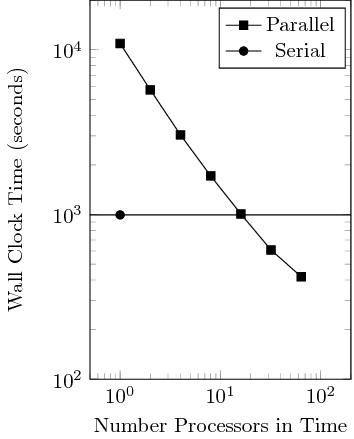
To test the performance, a strong scaling study is run. The spatial grid is fixed at 3201 degrees of freedom, and the spatial grid consists of 25,000 uniform timesteps. No spatial parallelization is used and the grid is fixed for all timesteps. The parallel in time solution is solved using XBraid’s multigrid reduction in time algorithm on 1, 2, 4, 16, 32, and 64 processors. The serial in time solution is run on a single processor using traditional sequential time stepping. The results are shown in figure below. Running the multigrid algorithm on a single processor takes about an order of magnitude longer to run on a single processor than the serial algorithm on a single processor. At 16 processors the multigrid algorithm the wall clock time is approximately the same for the serial algorithm as for the multigrid algorithm, and for 32 and 64 processors in time the wall clock is faster by about a factor of 2 for 64 processors.

Using 64 times as many processors results in a speedup factor of approximately 2. This is a fairly heavy computational cost for a slight speedup. For comparison, in the reference paper they achieved a speedup of approximately 10 times when using 256 times as many processors as their serial case when solving the heat equation in two dimensions. A similar increase in processors may be needed to increase the speedup factor of this code from 2 to 10. The choice of whether to use serial in time or parallel in time largely rests in the size of problem being solved, the amount of computing resources available, and the urgency of the problem being solved. Increasing the required number of timesteps will benefit the parallel in time algorithm provided enough extra resources are available.
There are many routes available for future work. First there are many optimizations that could be made to speed up the existing code base such as exploring the different multigrid cycles and finding the optimal load balancing. Ultimately those optimizations will probably only result in marginal gains per the reference paper. Allowing XBraid to prolong and restrict the spatial grid may be one of the more promising avenues of improvement.
Future work that is of interest to the authors of XBraid is the development of adaptive mesh refinement (AMR) in a parallel in time algorithm. A particular challenges with parallel-in-time AMR is the time subcylcing that occurs in spatial subdomains with sequential time stepping. This code base does not use spatial subdomains with AMR and so could provide an easier understanding of the coarsening and refining of the time domain.
This advances the solution forward by one time step. First some data is collected from the status struct, namely the start and stop time and the current timestep number. The timestep size \Delta t is calculated, and the step function from the HeatEquation is used to advance the solution.
In this function we initialize a vector at an arbitrary time. At this point we don't know anything about what the solution looks like, and we can really initialize to anything, so in this case use reinit to initialize the memory and set the values to zero.
Here we need to copy the vector u into the vector v. We do this by allocating a new vector, then reinitializing the deal.ii vector to the correct size. The deal.ii reinitialization sets every value to zero, so next we need to iterate over the vector u and copy the values to the new vector v.
Here we need to free the memory used by vector u. This is pretty simple since the deal.ii vector is stored inside the XBraid vector, so we just delete the XBraid vector u and it puts the deal.ii vector out of scope and releases its memory.
This is to perform an axpy type operation. That is to say we do y = \alpha x + \beta y. Fortunately deal.ii already has this operation built in to its vector class, so we get the reference to the vector y and call the sadd method.
This calculates the spatial norm using the l2 norm. According to XBraid, this could be just about any spatial norm but we'll keep it simple and used deal.ii vector's built in l2_norm method.
This function is called at various points depending on the access level specified when configuring the XBraid struct. This function is used to print out data during the run time, such as plots of the data. The status struct contains a ton of information about the simulation run. Here we get the current time and timestep number. The output_results function is called to plot the solution data. If the method of manufactured solutions is being used, then the error of this time step is computed and processed.
This calculates the size of buffer needed to pack the solution data into a linear buffer for transfer to another processor via MPI. We query the size of the data from the HeatEquation class and return the buffer size.
This function packs a linear buffer with data so that the buffer may be sent to another processor via MPI. The buffer is cast to a type we can work with. The first element of the buffer is the size of the buffer. Then we iterate over soltuion vector u and fill the buffer with our solution data. Finally we tell XBraid how much data we wrote.
This function unpacks a buffer that was recieved from a different processor via MPI. The size of the buffer is read from the first element, then we iterate over the size of the buffer and fill the values of solution vector u with the data in the buffer.
This struct contains all data that changes with time. For now this is just the solution data. When doing AMR this should probably include the triangulization, the sparsity patter, constraints, etc.
This struct contains all the data that is unchanging with time.
The HeatEquation class is describes the finite element solver for the heat equation. It contains all the functions needed to define the problem domain and advance the solution in time.
These were originally in the run() function but because I am splitting the run() function up into define and step they need to become member data
The RightHandSide class describes the RHS of the governing equations. In this case, it is the forcing function.
The BoundaryValues class describes the boundary conditions of the governing equations.
The RightHandSideMFG class describes the right hand side function when doing the method of manufactured solutions.
The InitialValuesMFG class describes the initial values when doing the method of manufactured solutions.
Provides the exact value for the manufactured solution. This is used for the boundary conditions as well.
Calculates the forcing function for the RightHandSide. See the documentation for the math.
Calculates the forcing function for the method of manufactured solutions. See the documentation for the math.
Calculates the boundary conditions, essentially zero everywhere.
Calculates the exact solution (and thus also boundary conditions) for the method of manufactured solutions.
Calculates the gradient of the exact solution for the method of manufactured solutions. See the documentation for the math.
Calculates the initial values for the method of manufactured solutions. See the documentation for the math.
We only initialize values in the manufactured solution case
If not the MFG solution case, a_vector is already zero'd so do nothing
We define the geometry here, this is called on each processor and doesn't change in time. Once doing AMR, this won't need to exist anymore.
Here we advance the solution forward in time. This is done the same way as in the loop in step-26's run function.
If we are doing the method of manufactured solutions then we set the boundary conditions to the exact solution. Otherwise the boundary conditions are zero.
This function computes the error for the time step when doing the method of manufactured solutions. First the exact values is calculated, then the difference per cell is computed for the various norms, and the error is computed. This is written out to a pretty table.
Compute the exact value for the manufactured solution case
The shared variables
in parallel, compute the filename give the basename [NOTE: dont call this before MPI is initialized.]
in parallel, close the file if nec., open it and check for success
if open() fails, we have problems, but it's better to try again later than to make believe it succeeded
in serial, filename is always cout
in serial, this does absolutely nothing
the common case is _open == true, which just returns s_pout
the uncommon cae: the file isn't opened, MPI may not be initialized, and the basename may not have been set
app hasn't set a basename yet, so set the default
if MPI not initialized, we cant open the file so return cout
MPI is initialized, so file must not be, so open it
finally, in case the open failed, return cout
This preprocessor macro is used on function arguments that are not used in the function. It is used to suppress compiler warnings.
Contains the current MPI processor ID.
Function to return the ostream to write out to. In MPI mode it returns a stream to a file named pout.<#> where <#> is the procID. This allows the user to write output from each processor to a separate file. In serial mode (no MPI), it returns the standard output.
Set up X-Braid
int nrelax = 1; int skip = 0;
int cfactor = 2;
int min_coarse = 10; int fmg = 0; int scoarsen = 0; int res = 0; int wrapper_tests = 0;
braid_SetMinCoarse( core, min_coarse ); braid_SetSkip(core, skip); braid_SetNRelax(core, -1, nrelax);
braid_SetCFactor(core, -1, cfactor);
Free the memory now that we are done
Clean up MPI MPI_Comm_free(&comm);
/* Create spatial communicator for wrapper-tests