 |
Reference documentation for deal.II version 9.3.3
|
 |
Reference documentation for deal.II version 9.3.3
|
This tutorial depends on step-49.
This program was contributed by Martin Kronbichler.
This tutorial program presents an advanced manifold class, TransfiniteInterpolationManifold, and how to work around its main disadvantage, the relatively high cost.
In many applications, the finite element mesh must be able to represent a relatively complex geometry. In the step-1, step-49, and step-53 tutorial programs, some techniques to generate grids available within the deal.II library have been introduced. Given a base mesh, deal.II is then able to create a finer mesh by subdividing the cells into children, either uniformly or only in selected parts of the computational domain. Besides the basic meshing capabilities collected in the GridGenerator namespace, deal.II also comes with interfaces to read in meshes generated by (quad- and hex-only) mesh generators using the functions of namespace GridIn, as for example demonstrated in step-5. A fundamental limitation of externally generated meshes is that the information provided by the generated cells in the mesh only consists of the position of the vertices and their connectivity, without the context of the underlying geometry that used to be available in the mesh generator that originally created this mesh. This becomes problematic once the mesh is refined within deal.II and additional points need to be placed. The step-54 tutorial program shows how to overcome this limitation by using CAD surfaces in terms of the OpenCASCADE library, and step-53 by providing the same kind of information programmatically from within the source code.
Within deal.II, the placement of new points during mesh refinement or for the definition of higher order mappings is controlled by manifold objects, see the manifold module for details. To give an example, consider the following situation of a two-dimensional annulus (with pictures taken from the manifold module). If we start with an initial mesh of 10 cells and refine the mesh three times globally without attaching any manifolds, we would obtain the following mesh:
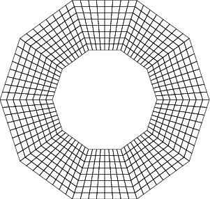
The picture looks like this because, by default, deal.II only knows where to put the vertices of child cells by averaging the locations of the vertices of the parent cell. This yields a polygonal domain whose faces are the edges of the original (coarse mesh) cells. Obviously, we must attach a curved description to the boundary faces of the triangulation to reproduce the circular shape upon mesh refinement, like in the following picture:
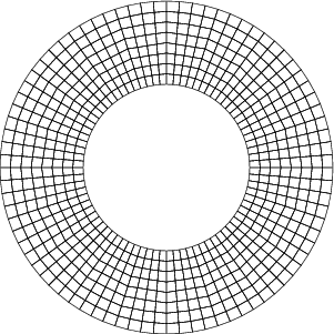
This is better: At least the inner and outer boundaries are now approaching real circles if we continue to refine the mesh. However, the mesh in this picture is still not optimal for an annulus in the sense that the interior lines from one cell to the next have kinks at certain vertices, and one would rather like to use the following mesh:
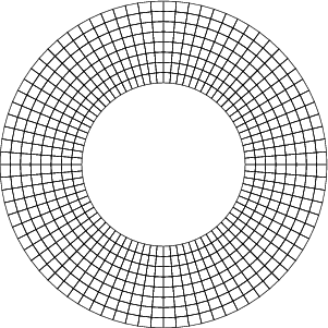
In this last (optimal) case, which is also the default produced by GridGenerator::hyper_shell(), the curved manifold description (in this case a polar manifold description) is applied not only to the boundary faces, but to the whole domain. Whenever the triangulation requests a new point, e.g., the mid point of the edges or the cells when it refines a cell into four children, it will place them along the respective mid points in the polar coordinate system. By contrast, the case above where only the boundary was subject to the polar manifold, only mid points along the boundary would be placed along the curved description, whereas mid points in the interior would be computed by suitable averages of the surrounding points in the Cartesian coordinate system (see the manifold module for more details).
At this point, one might assume that curved volume descriptions are the way to go. This is generally not wrong, though it is sometimes not so easy to describe how exactly this should work. Here are a couple of examples:
These simple examples make it clear that for many interesting cases we must step back from the desire to have an analytic curved description for the full volume: There will need to be some kind of information that leads to curvature also in the interior, but it must be possible to do this without actually writing down an explicit formula that describes the kind of geometry.
So what happens if we don't do anything at all in the interior and only describe the surface as a manifold? Sometimes, as in the ring shown above, the result is not terrible. But sometimes it is. Consider the case of a torus (e.g. generated with GridGenerator::torus()) with a TorusManifold object attached to the surface only, no additional manifolds on the interior cells and faces, and with six cells in toroidal direction before refinement. If the mesh is refined once, we would obtain the following mesh, shown with the upper half of the mesh clipped away:
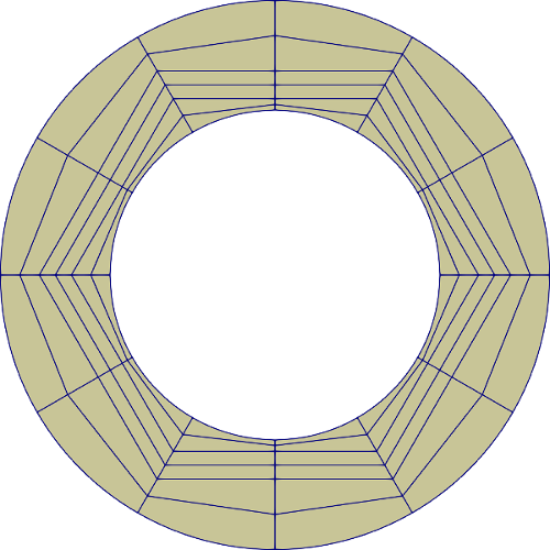
This is clearly sub-optimal. Indeed, if we had started with fewer than the six cells shown above in toroidal direction, the mapping actually inverts in some regions because the new points placed along interior cells intersect with the boundary as they are not following the circular shape along the toroidal direction. The simple case of a torus can still be fixed because we know that the toroidal direction follows a cylindrical coordinate system, so attaching a TorusManifold to the surface combined with CylindricalManifold with appropriate periodicity in toroidal direction applied to all interior entities would produce a high-quality mesh as follows, now shown with two top cells hidden:
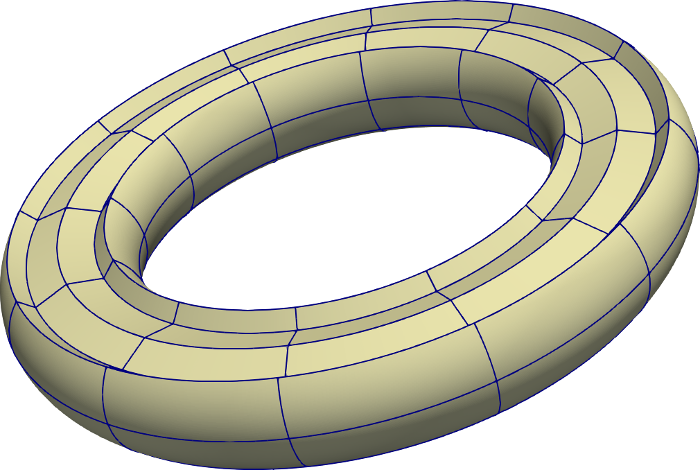
This mesh is pretty good, but obviously it is linked to a good description of the volume, which we lack in other cases. Actually, there is an imperfection also in this case, as we can see some unnatural kinks of two adjacent cells in the interior of the domain which are hidden by the top two boundary cells, as opposed to the following setup (the default manifolds applied by GridGenerator::torus() and using the TransfiniteInterpolationManifold):
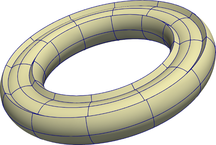
In order to find a better strategy, let us look at the two-dimensional disk again (that is also the base entity rotated along the toroidal direction in the torus). As we learned above, we can only apply the curved polar description to the boundary (or a rim of cells sufficiently far away from the origin) but must eventually transition to a straight description towards the disk's center. If we use a flat manifold in the interior of the cells (i.e., one in which new vertices are created by averaging of the adjacent existing ones) and a polar manifold only for the boundary of the disk, we get the following mesh upon four global refinements:
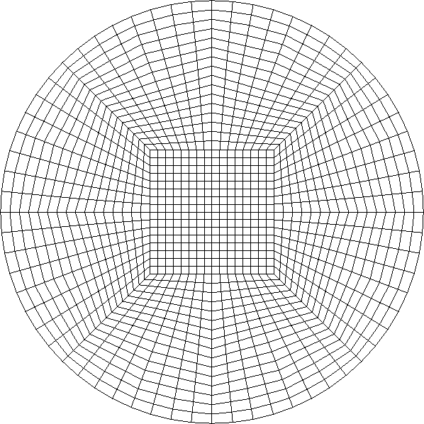
That's not a terrible mesh. At the same time, if you know that the original coarse mesh consisted of a single square in the middle, with four caps around it, then it's not hard to see every refinement step that happened to this mesh to get the picture above.
While the triangulation class of deal.II tries to propagate information from the boundary into the interior when creating new points, the reach of this algorithm is limited:

The picture above highlights those cells on the disk that are touching the boundary and where boundary information could in principle be taken into account when only looking at a single cell at the time. Clearly, the area where some curvature can be taken into account gets more limited as the mesh is refined, thus creating the seemingly irregular spots in the mesh: When computing the center of any one of the boundary cells in the leftmost picture, the ideal position is the mid point between the outer circle and the cell in the middle. This is exactly what is used for the first refinement step in the Triangulation class. However, for the second refinement all interior edges as well as the interior cell layers can only add points according to a flat manifold description.
At this point, we realize what would be needed to create a better mesh: For all new points in any child cell that is created within the red shaded layer on the leftmost picture, we want to compute the interpolation with respect to the curvature in the area covered by the respective coarse cell. This is achieved by adding the class TransfiniteInterpolationManifold to the highlighted cells of the coarse grid in the leftmost panel of the figure above. This class adheres to the general manifold interfaces, i.e., given any set of points within its domain of definition, it can compute weighted averages conforming to the manifold (using a formula that will be given in a minute). These weighted averages are used whenever the mesh is refined, or when a higher order mapping (such as MappingQGeneric or MappingC1) is evaluated on a given cell subject to this manifold. Using this manifold on the shaded cells of the coarse grid of the disk (i.e., not only in the outer-most layer of cells) produces the following mesh upon four global steps of refinement:
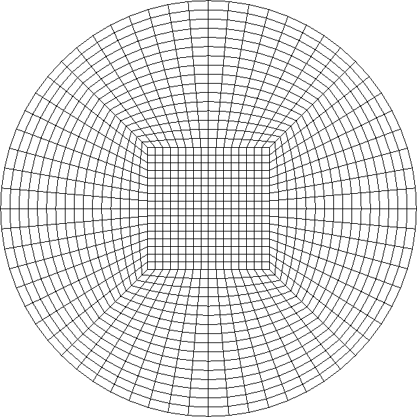
There are still some kinks in the lines of this mesh, but they are restricted to the faces between coarse mesh cells, whereas the rest of the mesh is about as smooth as one would like. Indeed, given a straight-sided central cell, this representation is the best possible one as all mesh cells follow a smooth transition from the straight sides in the square block in the interior to the circular shape on the boundary. (One could possibly do a bit better by allowing some curvature also in the central square block, that eventually vanishes as the center is approached.)
In the simple case of a disk with one curved and three straight edges, we can explicitly write down how to achieve the blending of the shapes. For this, it is useful to map the physical cell, like the top one, back to the reference coordinate system (\xi,\eta)\in (0,1)^2 where we compute averages between certain points. If we were to use a simple bilinear map spanned by four vertices (x_0,y_0), (x_1,y_1), (x_2,y_2), (x_3, y_3), the image of a point (\xi, \eta)\in (0,1)^2 would be
\begin{align*} (x,y) = (1-\xi)(1-\eta) (x_0,y_0) + \xi(1-\eta) (x_1,y_1) + (1-\xi)\eta (x_2,y_2) + \xi\eta (x_3,y_3). \end{align*}
For the case of the curved surface, we want to modify this formula. For the top cell of the coarse mesh of the disk, we can assume that the points (x_0,y_0) and (x_1,y_1) sit along the straight line at the lower end and the points (x_2,y_2) and (x_3,y_3) are connected by a quarter circle along the top. We would then map a point (\xi, \eta) as
\begin{align*} (x,y) = (1-\eta) \big[(1-\xi) (x_0,y_0) + \xi (x_1,y_1)\big] + \eta \mathbf{c}_3(\xi), \end{align*}
where \mathbf{c}_3(\xi) is a curve that describes the (x,y) coordinates of the quarter circle in terms of an arclength parameter \xi\in (0,1). This represents a linear interpolation between the straight lower edge and the curved upper edge of the cell, and is the basis for the picture shown above.
This formula is easily generalized to the case where all four edges are described by a curve rather than a straight line. We call the four functions, parameterized by a single coordinate \xi or \eta in the horizontal and vertical directions, \mathbf{c}_0, \mathbf{c}_1, \mathbf{c}_2, \mathbf{c}_3 for the left, right, lower, and upper edge of a quadrilateral, respectively. The interpolation then reads
\begin{align*} (x,y) =& (1-\xi)\mathbf{c}_0(\eta) + \xi \mathbf{c}_1(\eta) +(1-\eta)\mathbf{c}_2(\xi) + \eta \mathbf{c}_3(\xi)\\ &-\big[(1-\xi)(1-\eta) (x_0,y_0) + \xi(1-\eta) (x_1,y_1) + (1-\xi)\eta (x_2,y_2) + \xi\eta (x_3,y_3)\big]. \end{align*}
This formula assumes that the boundary curves match and coincide with the vertices (x_0,y_0), (x_1,y_1), (x_2,y_2), (x_3, y_3), e.g. \mathbf{c}_0(0) = (x_0,y_0) or \mathbf{c}_0(1) = (x_2,y_2). The subtraction of the bilinear interpolation in the second line of the formula makes sure that the prescribed curves are followed exactly on the boundary: Along each of the four edges, we need to subtract the contribution of the two adjacent edges evaluated in the corners, which is then simply a vertex position. It is easy to check that the formula for the circle above is reproduced if three of the four curves \mathbf{c}_i are straight and thus coincide with the bilinear interpolation.
This formula, called transfinite interpolation, was introduced in 1973 by Gordon and Hall. Even though transfinite interpolation essentially only represents a linear blending of the bounding curves, the interpolation exactly follows the boundary curves for each real number \xi\in (0,1) or \eta\in (0,1), i.e., it interpolates in an infinite number of points, which was the original motivation to label this variant of interpolation a transfinite one by Gordon and Hall. Another interpretation is that the transfinite interpolation interpolates from the left and right and the top and bottom linearly, from which we need to subtract the bilinear interpolation to ensure a unit weight in the interior of the domain.
The transfinite interpolation is easily generalized to three spatial dimensions. In that case, the interpolation allows to blend 6 different surface descriptions for any of the quads of a three-dimensional cell and 12 edge descriptions for the lines of a cell. Again, to ensure a consistent map, it is necessary to subtract the contribution of edges and add the contribution of vertices again to make the curves follow the prescribed surface or edge description. In the three-dimensional case, it is also possible to use a transfinite interpolation from a curved edge both into the adjacent faces and the adjacent cells.
The interpolation of the transfinite interpolation in deal.II is general in the sense that it can deal with arbitrary curves. It will evaluate the curves in terms of their original coordinates of the d-dimensional space but with one (or two, in the case of edges in 3D) coordinate held fixed at 0 or 1 to ensure that any other manifold class, including CAD files if desired, can be applied out of the box. Transfinite interpolation is a standard ingredient in mesh generators, so the main strength of the integration of this feature within the deal.II library is to enable it during adaptive refinement and coarsening of the mesh, and for creating higher-degree mappings that use manifolds to insert additional points beyond the mesh vertices.
As a final remark on transfinite interpolation, we mention that the mesh refinement strategies in deal.II in absence of a volume manifold description are also based on the weights of the transfinite interpolation and optimal in that sense. The difference is that the default algorithm sees only one cell at a time, and so will apply the optimal algorithm only on those cells touching the curved manifolds. In contrast, using the transfinite mapping on entire patches of cells (originating from one coarser cell) allows to use the transfinite interpolation method in a way that propagates information from the boundary to cells far away.
A mesh with a transfinite manifold description is typically set up in two steps. The first step is to create a coarse mesh (or read it in from a file) and to attach a curved manifold to some of the mesh entities. For the above example of the disk, we attach a polar manifold to the faces along the outer circle (this is done automatically by GridGenerator::hyper_ball()). Before we start refining the mesh, we then assign a TransfiniteInterpolationManifold to all interior cells and edges of the mesh, which of course needs to be based on some manifold id that we have assigned to those entities (everything except the circle on the boundary). It does not matter whether we also assign a TransfiniteInterpolationManifold to the inner square of the disk or not because the transfinite interpolation on a coarse cell with straight edges (or flat faces in 3d) simply yields subdivided children with straight edges (flat faces).
Later, when the mesh is refined or when a higher-order mapping is set up based on this mesh, the cells will query the underlying manifold object for new points. This process takes a set of surrounding points, for example the four vertices of a two-dimensional cell, and a set of weights to each of these points, for definition a new point. For the mid point of a cell, each of the four vertices would get weight 0.25. For the transfinite interpolation manifold, the process of building weighted sums requires some serious work. By construction, we want to combine the points in terms of the reference coordinates \xi and \eta (or \xi, \eta, \zeta in 3D) of the surrounding points. However, the interface of the manifold classes in deal.II does not get the reference coordinates of the surrounding points (as they are not stored globally) but rather the physical coordinates only. Thus, the first step the transfinite interpolation manifold has to do is to invert the mapping and find the reference coordinates within one of the coarse cells of the transfinite interpolation (e.g. one of the four shaded coarse-grid cells of the disk mesh above). This inversion is done by a Newton iteration (or rather, finite-difference based Newton scheme combined with Broyden's method) and queries the transfinite interpolation according to the formula above several times. Each of these queries in turn might call an expensive manifold, e.g. a spherical description of a ball, and be expensive on its own. Since the Manifold interface class of deal.II only provides a set of points, the transfinite interpolation initially does not even know to which coarse grid cell the set of surrounding points belong to and needs to search among several cells based on some heuristics. In terms of charts, one could describe the implementation of the transfinite interpolation as an atlas-based implementation: Each cell of the initial coarse grid of the triangulation represents a chart with its own reference space, and the surrounding manifolds provide a way to transform from the chart space (i.e., the reference cell) to the physical space. The collection of the charts of the coarse grid cells is an atlas, and as usual, the first thing one does when looking up something in an atlas is to find the right chart.
Once the reference coordinates of the surrounding points have been found, a new point in the reference coordinate system is computed by a simple weighted sum. Finally, the reference point is inserted into the formula for the transfinite interpolation, which gives the desired new point.
In a number of cases, the curved manifold is not only used during mesh refinement, but also to ensure a curved representation of boundaries within the cells of the computational domain. This is a necessity to guarantee high-order convergence for high-order polynomials on complex geometries anyway, but sometimes an accurate geometry is also desired with linear shape functions. This is often done by polynomial descriptions of the cells and called the isoparametric concept if the polynomial degree to represent the curved mesh elements is the same as the degree of the polynomials for the numerical solution. If the degree of the geometry is higher or lower than the solution, one calls that a super- or sub-parametric geometry representation, respectively. In deal.II, the standard class for polynomial representation is MappingQGeneric. If, for example, this class is used with polynomial degree 4 in 3D, a total of 125 (i.e., (4+1)^3) points are needed for the interpolation. Among these points, 8 are the cell's vertices and already available from the mesh, but the other 117 need to be provided by the manifold. In case the transfinite interpolation manifold is used, we can imagine that going through the pull-back into reference coordinates of some yet to be determined coarse cell, followed by subsequent push-forward on each of the 117 points, is a lot of work and can be very time consuming.
What makes things worse is that the structure of many programs is such that the mapping is queried several times independently for the same cell. Its primary use is in the assembly of the linear system, i.e., the computation of the system matrix and the right hand side, via the mapping argument of the FEValues object. However, also the interpolation of boundary values, the computation of numerical errors, writing the output, and evaluation of error estimators must involve the same mapping to ensure a consistent interpretation of the solution vectors. Thus, even a linear stationary problem that is solved once will evaluate the points of the mapping several times. For the cubic case in 3D mentioned above, this means computing 117 points per cell by an expensive algorithm many times. The situation is more pressing for nonlinear or time-dependent problems where those operations are done over and over again.
As the manifold description via a transfinite interpolation can easily be hundreds of times more expensive than a similar query on a flat manifold, it makes sense to compute the additional points only once and use them in all subsequent calls. The deal.II library provides the class MappingQCache for exactly this purpose. The cache is typically not overly big compared to the memory consumed by a system matrix, as will become clear when looking at the results of this tutorial program. The usage of MappingQCache is simple: Once the mesh has been set up (or changed during refinement), we call MappingQCache::initialize() with the desired triangulation as well as a desired mapping as arguments. The initialization then goes through all cells of the mesh and queries the given mapping for its additional points. Those get stored for an identifier of the cell so that they can later be returned whenever the mapping computes some quantities related to the cell (like the Jacobians of the map between the reference and physical coordinates).
As a final note, we mention that the TransfiniteInterpolationManifold also makes the refinement of the mesh more expensive. In this case, the MappingQCache does not help because it would compute points that can subsequently not be re-used; there currently does not exist a more efficient mechanism in deal.II. However, the mesh refinement contains many other expensive steps as well, so it is not as big as an issue compared to the rest of the computation. It also only happens at most once per time step or nonlinear iteration.
In this tutorial program, the usage of TransfiniteInterpolationManifold is exemplified in combination with MappingQCache. The test case is relatively simple and takes up the solution stages involved in many typical programs, e.g., the step-6 tutorial program. As a geometry, we select one prototype use of TransfiniteInterpolationManifold, namely a setup involving a spherical ball that is in turn surrounded by a cube. Such a setup would be used, for example, for a spherical inclusion embedded in a background medium, and if that inclusion has different material properties that require that the interface between the two materials needs to be tracked by element interfaces. A visualization of the grid is given here:
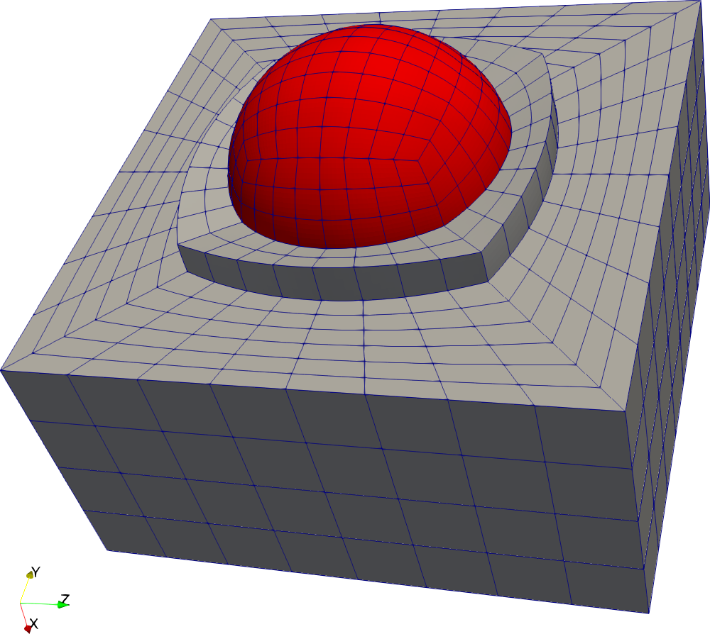
For this case, we want to attach a spherical description to the surface inside the domain and use the transfinite interpolation to smoothly switch to the straight lines of the outer cube and the cube at the center of the ball.
Within the program, we will follow a typical flow in finite element programs, starting from the setup of DoFHandler and sparsity patterns, the assembly of a linear system for solving the Poisson equation with a jumping coefficient, its solution with a simple iterative method, computation of some numerical error with VectorTools::integrate_difference() as well as an error estimator. We record timings for each section and run the code twice. In the first run, we hand a MappingQGeneric object to each stage of the program separately, where points get re-computed over and over again. In the second run, we use MappingQCache instead.
The include files for this tutorial are essentially the same as in step-6. Importantly, the TransfiniteInterpolationManifold class we will be using is provided by deal.II/grid/manifold_lib.h.
The only new include file is the one for the MappingQCache class.
In this tutorial program, we want to solve the Poisson equation with a coefficient that jumps along a sphere of radius 0.5, and using a constant right hand side of value f(\mathbf{x}) = -3. (This setup is similar to step-5 and step-6, but the concrete values for the coefficient and the right hand side are different.) Due to the jump in the coefficient, the analytical solution must have a kink where the coefficient switches from one value to the other. To keep things simple, we select an analytical solution that is quadratic in all components, i.e., u(x,y,z) = x^2 + y^2 + z^2 in the ball of radius 0.5 and u(x,y,z) = 0.1(x^2 + y^2 + z^2) + 0.25-0.025 in the outer part of the domain. This analytical solution is compatible with the right hand side in case the coefficient is 0.5 in the inner ball and 5 outside. It is also continuous along the circle of radius 0.5.
The implementation of the Poisson problem is very similar to what we used in the step-5 tutorial program. The two main differences are that we pass a mapping object to the various steps in the program in order to switch between two mapping representations as explained in the introduction, and the timer object (of type TimerOutput) that will be used for measuring the run times in the various cases. (The concept of mapping objects was first introduced in step-10 and step-11, in case you want to look up the use of these classes.)
In the constructor, we set up the timer object to record wall times but be quiet during the normal execution. We will query it for timing details in the PoissonProblem::run() function. Furthermore, we select a relatively high polynomial degree of three for the finite element in use.
The next function presents the typical usage of TransfiniteInterpolationManifold. The first step is to create the desired grid, which can be done by composition of two grids from GridGenerator. The inner ball mesh is simple enough: We run GridGenerator::hyper_cube() centered at the origin with radius 0.5 (third function argument). The second mesh is more interesting and constructed as follows: We want to have a mesh that is spherical in the interior but flat on the outer surface. Furthermore, the mesh topology of the inner ball should be compatible with the outer grid in the sense that their vertices coincide so as to allow the two grid to be merged. The grid coming out of GridGenerator::hyper_shell fulfills the requirements on the inner side in case it is created with 2d coarse cells (6 coarse cells in 3D which we are going to use) – this is the same number of cells as there are boundary faces for the ball. For the outer surface, we use the fact that the 6 faces on the surface of the shell without a manifold attached would degenerate to the surface of a cube. What we are still missing is the radius of the outer shell boundary. Since we desire a cube of extent [-1, 1] and the 6-cell shell puts its 8 outer vertices at the 8 opposing diagonals, we must translate the points (\pm 1, \pm 1, \pm 1) into a radius: Clearly, the radius must be \sqrt{d} in d dimensions, i.e., \sqrt{3} for the three-dimensional case we want to consider.
Thus, we have a plan: After creating the inner triangulation for the ball and the one for the outer shell, we merge those two grids but remove all manifolds that the functions in GridGenerator may have set from the resulting triangulation, to ensure that we have full control over manifolds. In particular, we want additional points added on the boundary during refinement to follow a flat manifold description. To start the process of adding more appropriate manifold ids, we assign the manifold id 0 to all mesh entities (cells, faces, lines), which will later be associated with the TransfiniteInterpolationManifold. Then, we must identify the faces and lines that are along the sphere of radius 0.5 and mark them with a different manifold id, so as to then assign a SphericalManifold to those. We will choose the manifold id of 1. Since we have thrown away all manifolds that pre-existed after calling GridGenerator::hyper_ball(), we manually go through the cells of the mesh and all their faces. We have found a face on the sphere if all four vertices have a radius of 0.5, or, as we write in the program, have r^2-0.25 \approx 0. Note that we call cell->face(f)->set_all_manifold_ids(1) to set the manifold id both on the faces and the surrounding lines. Furthermore, we want to distinguish the cells inside the ball and outside the ball by a material id for visualization, corresponding to the picture in the introduction.
With all cells, faces and lines marked appropriately, we can attach the Manifold objects to those numbers. The entities with manifold id 1 will get a spherical manifold, whereas the other entities, which have the manifold id 0, will be assigned the TransfiniteInterpolationManifold. As mentioned in the introduction, we must explicitly initialize the manifold with the current mesh using a call to TransfiniteInterpolationManifold::initialize() in order to pick up the coarse mesh cells and the manifolds attached to the boundaries of those cells. We also note that the manifold objects we create locally in this function are allowed to go out of scope (as they do at the end of the function scope), because the Triangulation object internally copies them.
With all manifolds attached, we will finally go about and refine the mesh a few times to create a sufficiently large test case.
The following function is well-known from other tutorials in that it enumerates the degrees of freedom, creates a constraint object and sets up a sparse matrix for the linear system. The only thing worth mentioning is the fact that the function receives a reference to a mapping object that we then pass to the VectorTools::interpolate_boundary_values() function to ensure that our boundary values are evaluated on the high-order mesh used for assembly. In the present example, it does not really matter because the outer surfaces are flat, but for curved outer cells this leads to more accurate approximation of the boundary values.
The function that assembles the linear system is also well known from the previous tutorial programs. One thing to note is that we set the number of quadrature points to the polynomial degree plus two, not the degree plus one as in most other tutorials. This is because we expect some extra accuracy as the mapping also involves a degree one more than the polynomials for the solution.
The only somewhat unusual code in the assembly is the way we compute the cell matrix. Rather than using three nested loop over the quadrature point index, the row, and the column of the matrix, we first collect the derivatives of the shape function, multiplied by the square root of the product of the coefficient and the integration factor JxW in a separate matrix partial_matrix. To compute the cell matrix, we then execute cell_matrix = partial_matrix * transpose(partial_matrix) in the line partial_matrix.mTmult(cell_matrix, partial_matrix);. To understand why this works, we realize that the matrix-matrix multiplication performs a summation over the columns of partial_matrix. If we denote the coefficient by a(\mathbf{x}_q), the entries in the temporary matrix are \sqrt{\text{det}(J) w_q a(x)} \frac{\partial \varphi_i(\boldsymbol
\xi_q)}{\partial x_k}. If we take the product of the ith row with the jth column of that matrix, we compute a nested sum involving \sum_q \sum_{k=1}^d \sqrt{\text{det}(J) w_q a(x)} \frac{\partial
\varphi_i(\boldsymbol \xi_q)}{\partial x_k} \sqrt{\text{det}(J) w_q a(x)}
\frac{\partial \varphi_j(\boldsymbol \xi_q)}{\partial x_k} = \sum_q
\sum_{k=1}^d\text{det}(J) w_q a(x)\frac{\partial \varphi_i(\boldsymbol
\xi_q)}{\partial x_k} \frac{\partial \varphi_j(\boldsymbol
\xi_q)}{\partial x_k}, which is exactly the terms needed for the bilinear form of the Laplace equation.
The reason for choosing this somewhat unusual scheme is due to the heavy work involved in computing the cell matrix for a relatively high polynomial degree in 3D. As we want to highlight the cost of the mapping in this tutorial program, we better do the assembly in an optimized way in order to not chase bottlenecks that have been solved by the community already. Matrix-matrix multiplication is one of the best optimized kernels in the HPC context, and the FullMatrix::mTmult() function will call into those optimized BLAS functions. If the user has provided a good BLAS library when configuring deal.II (like OpenBLAS or Intel's MKL), the computation of the cell matrix will execute close to the processor's peak arithmetic performance. As a side note, we mention that despite an optimized matrix-matrix multiplication, the current strategy is sub-optimal in terms of complexity as the work to be done is proportional to (p+1)^9 operations for degree p (this also applies to the usual evaluation with FEValues). One could compute the cell matrix with \mathcal O((p+1)^7) operations by utilizing the tensor product structure of the shape functions, as is done by the matrix-free framework in deal.II. We refer to step-37 and the documentation of the tensor-product-aware evaluators FEEvaluation for details on how an even more efficient cell matrix computation could be realized.
For solving the linear system, we pick a simple Jacobi-preconditioned conjugate gradient solver, similar to the settings in the early tutorials.
In the next function we do various post-processing steps with the solution, all of which involve the mapping in one way or the other.
The first operation we do is to write the solution as well as the material ids to a VTU file. This is similar to what was done in many other tutorial programs. The new ingredient presented in this tutorial program is that we want to ensure that the data written to the file used for visualization is actually a faithful representation of what is used internally by deal.II. That is because most of the visualization data formats only represent cells by their vertex coordinates, but have no way of representing the curved boundaries that are used in deal.II when using higher order mappings – in other words, what you see in the visualization tool is not actually what you are computing on. (The same, incidentally, is true when using higher order shape functions: Most visualization tools only render bilinear/trilinear representations. This is discussed in detail in DataOut::build_patches().)
So we need to ensure that a high-order representation is written to the file. We need to consider two particular topics. Firstly, we tell the DataOut object via the DataOutBase::VtkFlags that we intend to interpret the subdivisions of the elements as a high-order Lagrange polynomial rather than a collection of bilinear patches. Recent visualization programs, like ParaView version 5.5 or newer, can then render a high-order solution (see a wiki page for more details). Secondly, we need to make sure that the mapping is passed to the DataOut::build_patches() method. Finally, the DataOut class only prints curved faces for boundary cells by default, so we need to ensure that also inner cells are printed in a curved representation via the mapping.
The next operation in the postprocessing function is to compute the L_2 and H^1 errors against the analytical solution. As the analytical solution is a quadratic polynomial, we expect a very accurate result at this point. If we were solving on a simple mesh with planar faces and a coefficient whose jumps are aligned with the faces between cells, then we would expect the numerical result to coincide with the analytical solution up to roundoff accuracy. However, since we are using deformed cells following a sphere, which are only tracked by polynomials of degree 4 (one more than the degree for the finite elements), we will see that there is an error around 10^{-7}. We could get more accuracy by increasing the polynomial degree or refining the mesh.
The final post-processing operation we do here is to compute an error estimate with the KellyErrorEstimator. We use the exact same settings as in the step-6 tutorial program, except for the fact that we also hand in the mapping to ensure that errors are evaluated along the curved element, consistent with the remainder of the program. However, we do not really use the result here to drive a mesh adaptation step (that would refine the mesh around the material interface along the sphere), as the focus here is on the cost of this operation.
Finally, we define the run() function that controls how we want to execute this program (which is called by the main() function in the usual way). We start by calling the create_grid() function that sets up our geometry with the appropriate manifolds. We then run two instances of a solver chain, starting from the setup of the equations, the assembly of the linear system, its solution with a simple iterative solver, and the postprocessing discussed above. The two instances differ in the way they use the mapping. The first uses a conventional MappingQGeneric mapping object which we initialize to a degree one more than we use for the finite element – after all, we expect the geometry representation to be the bottleneck as the analytic solution is only a quadratic polynomial. (In reality, things are interlinked to quite some extent because the evaluation of the polynomials in real coordinates involves the mapping of a higher-degree polynomials, which represent some smooth rational functions. As a consequence, higher-degree polynomials still pay off, so it does not make sense to increase the degree of the mapping further.) Once the first pass is completed, we let the timer print a summary of the compute times of the individual stages.
For the second instance, we instead set up the MappingQCache class. Its use is very simple: After constructing it (with the degree, given that we want it to show the correct degree functionality in other contexts), we fill the cache via the MappingQCache::initialize() function. At this stage, we specify which mapping we want to use (obviously, the same MappingQGeneric as previously in order to repeat the same computations) for the cache, and then run through the same functions again, now handing in the modified mapping. In the end, we again print the accumulated wall times since the reset to see how the times compare to the original setting.
If we run the three-dimensional version of this program with polynomials of degree three, we get the following program output:
Before discussing the timings, we look at the memory consumption for the MappingQCache object: Our program prints that it utilizes 23 MB of memory. If we relate this number to the memory consumption of a single (solution or right hand side) vector, which is 1.5 MB (namely, 181,609 elements times 8 bytes per entry in double precision), or to the memory consumed by the system matrix and the sparsity pattern (which is 274 MB), we realize that it is not an overly heavy data structure, given its benefits.
With respect to the timers, we see a clear improvement in the overall run time of the program by a factor of 2.7. If we disregard the iterative solver, which is the same in both cases (and not optimal, given the simple preconditioner we use, and the fact that sparse matrix-vector products waste operations for cubic polynomials), the advantage is a factor of almost 5. This is pretty impressive for a linear stationary problem, and cost savings would indeed be much more prominent for time-dependent and nonlinear problems where assembly is called several times. If we look into the individual components, we get a clearer picture of what is going on and why the cache is so efficient: In the MappingQGeneric case, essentially every operation that involves a mapping take at least 5 seconds to run. The norm computation runs two VectorTools::integrate_difference() functions, which each take almost 5 seconds. (The computation of constraints is cheaper because it only evaluates the mapping in cells at the boundary for the interpolation of boundary conditions.) If we compare these 5 seconds to the time it takes to fill the MappingQCache, which is 5.2 seconds (for all cells, not just the active ones), it becomes obvious that the computation of the mapping support points dominates over everything else in the MappingQGeneric case. Perhaps the most striking result is the time for the error estimator, labeled "Compute error estimator", where the MappingQGeneric implementation takes 17.3 seconds and the MappingQCache variant less than 0.5 seconds. The reason why the former is so expensive (three times more expensive than the assembly, for instance) is that the error estimation involves evaluation of quantities over faces, where each face in the mesh requests additional points of the mapping that in turn go through the very expensive TransfiniteInterpolationManifold class. As there are six faces per cell, this happens much more often than in assembly. Again, MappingQCache nicely eliminates the repeated evaluation, aggregating all the expensive steps involving the manifold in a single initialization call that gets repeatedly used.