 |
Reference documentation for deal.II version 9.3.3
|
 |
Reference documentation for deal.II version 9.3.3
|
This tutorial depends on step-4.
| Table of contents | |
|---|---|
This program was contributed by Toby D. Young and Wolfgang Bangerth.
The problem we want to solve in this example is an eigenspectrum problem. Eigenvalue problems appear in a wide context of problems, for example in the computation of electromagnetic standing waves in cavities, vibration modes of drum membranes, or oscillations of lakes and estuaries. One of the most enigmatic applications is probably the computation of stationary or quasi-static wave functions in quantum mechanics. The latter application is what we would like to investigate here, though the general techniques outlined in this program are of course equally applicable to the other applications above.
Eigenspectrum problems have the general form
\begin{align*} L \Psi &= \varepsilon \Psi \qquad &&\text{in}\ \Omega\quad, \\ \Psi &= 0 &&\text{on}\ \partial\Omega\quad, \end{align*}
where the Dirichlet boundary condition on \Psi=\Psi(\mathbf x) could also be replaced by Neumann or Robin conditions; L is an operator that generally also contains differential operators.
Under suitable conditions, the above equations have a set of solutions \Psi_\ell,\varepsilon_\ell, \ell\in {\cal I}, where \cal I can be a finite or infinite set (and in the latter case it may be a discrete or sometimes at least in part a continuous set). In either case, let us note that there is no longer just a single solution, but a set of solutions (the various eigenfunctions and corresponding eigenvalues) that we want to compute. The problem of numerically finding all eigenvalues (eigenfunctions) of such eigenvalue problems is a formidable challenge. In fact, if the set \cal I is infinite, the challenge is of course intractable. Most of the time however we are really only interested in a small subset of these values (functions); and fortunately, the interface to the SLEPc library that we will use for this tutorial program allows us to select which portion of the eigenspectrum and how many solutions we want to solve for.
In this program, the eigenspectrum solvers we use are classes provided by deal.II that wrap around the linear algebra implementation of the SLEPc library; SLEPc itself builds on the PETSc library for linear algebra contents.
The basic equation of stationary quantum mechanics is the Schrödinger equation which models the motion of particles in an external potential V(\mathbf x). The particle is described by a wave function \Psi(\mathbf x) that satisfies a relation of the (nondimensionalized) form
\begin{align*} [-\Delta + V(\mathbf x)] \Psi(\mathbf x) &= \varepsilon \Psi(\mathbf x) \qquad &&\text{in}\ \Omega\quad, \\ \Psi &= 0 &&\text{on}\ \partial\Omega\quad. \end{align*}
As a consequence, this particle can only exist in a certain number of eigenstates that correspond to the energy eigenvalues \varepsilon_\ell admitted as solutions of this equation. The orthodox (Copenhagen) interpretation of quantum mechanics posits that, if a particle has energy \varepsilon_\ell then the probability of finding it at location \mathbf x is proportional to |\Psi_\ell(\mathbf x)|^2 where \Psi_\ell is the eigenfunction that corresponds to this eigenvalue.
In order to numerically find solutions to this equation, i.e. a set of pairs of eigenvalues/eigenfunctions, we use the usual finite element approach of multiplying the equation from the left with test functions, integrating by parts, and searching for solutions in finite dimensional spaces by approximating \Psi(\mathbf x)\approx\Psi_h(\mathbf x)=\sum_{j}\phi_j(\mathbf x)\tilde\psi_j, where \tilde\psi is a vector of expansion coefficients. We then immediately arrive at the following equation that discretizes the continuous eigenvalue problem:
\sum_j [(\nabla\phi_i, \nabla\phi_j)+(V(\mathbf x)\phi_i,\phi_j)] \tilde{\psi}_j = \varepsilon_h \sum_j (\phi_i, \phi_j) \tilde{\psi}_j\quad.
In matrix and vector notation, this equation then reads:
A \tilde{\Psi} = \varepsilon_h M \tilde{\Psi} \quad,
where A is the stiffness matrix arising from the differential operator L, and M is the mass matrix. The solution to the eigenvalue problem is an eigenspectrum \varepsilon_{h,\ell}, with associated eigenfunctions \Psi_\ell=\sum_j \phi_j\tilde{\psi}_j.
In this program, we use Dirichlet boundary conditions for the wave function \Psi. What this means, from the perspective of a finite element code, is that only the interior degrees of freedom are real degrees of freedom: the ones on the boundary are not free but are forced to have a zero value, after all. On the other hand, the finite element method gains much of its power and simplicity from the fact that we just do the same thing on every cell, without having to think too much about where a cell is, whether it bounds on a less refined cell and consequently has a hanging node, or is adjacent to the boundary. All such checks would make the assembly of finite element linear systems unbearably difficult to write and even more so to read.
Consequently, of course, when you distribute degrees of freedom with your DoFHandler object, you don't care whether some of the degrees of freedom you enumerate are at a Dirichlet boundary. They all get numbers. We just have to take care of these degrees of freedom at a later time when we apply boundary values. There are two basic ways of doing this (either using MatrixTools::apply_boundary_values() after assembling the linear system, or using AffineConstraints::distribute_local_to_global() during assembly; see the constraints module for more information), but both result in the same: a linear system that has a total number of rows equal to the number of all degrees of freedom, including those that lie on the boundary. However, degrees of freedom that are constrained by Dirichlet conditions are separated from the rest of the linear system by zeroing out the corresponding row and column, putting a single positive entry on the diagonal, and the corresponding Dirichlet value on the right hand side.
If you assume for a moment that we had renumbered degrees of freedom in such a way that all of those on the Dirichlet boundary come last, then the linear system we would get when solving a regular PDE with a right hand side would look like this:
\begin{align*} \begin{pmatrix} A_i & 0 \\ 0 & D_b \end{pmatrix} \begin{pmatrix} U_i \\ U_b \end{pmatrix} = \begin{pmatrix} F_i \\ F_b \end{pmatrix}. \end{align*}
Here, subscripts i and b correspond to interior and boundary degrees of freedom, respectively. The interior degrees of freedom satisfy the linear system A_i U_i=F_i which yields the correct solution in the interior, and boundary values are determined by U_b = D_b^{-1} F_b where D_b is a diagonal matrix that results from the process of eliminating boundary degrees of freedom, and F_b is chosen in such a way that U_{b,j}=D_{b,jj}^{-1} F_{b,j} has the correct boundary values for every boundary degree of freedom j. (For the curious, the entries of the matrix D_b result from adding modified local contributions to the global matrix where for the local matrices the diagonal elements, if non-zero, are set to their absolute value; otherwise, they are set to the average of absolute values of the diagonal. This process guarantees that the entries of D_b are positive and of a size comparable to the rest of the diagonal entries, ensuring that the resulting matrix does not incur unreasonable losses of accuracy due to roundoff involving matrix entries of drastically different size. The actual values that end up on the diagonal are difficult to predict and you should treat them as arbitrary and unpredictable, but positive.)
For "regular" linear systems, this all leads to the correct solution. On the other hand, for eigenvalue problems, this is not so trivial. There, eliminating boundary values affects both matrices A and M that we will solve with in the current tutorial program. After elimination of boundary values, we then receive an eigenvalue problem that can be partitioned like this:
\begin{align*} \begin{pmatrix} A_i & 0 \\ 0 & D_A \end{pmatrix} \begin{pmatrix} \tilde\Psi_i \\ \tilde\Psi_b \end{pmatrix} = \epsilon_h \begin{pmatrix} M_i & 0 \\ 0 & D_M \end{pmatrix} \begin{pmatrix} \tilde\Psi_i \\ \tilde\Psi_b \end{pmatrix}. \end{align*}
This form makes it clear that there are two sets of eigenvalues: the ones we care about, and spurious eigenvalues from the separated problem
D_A \tilde \Psi_b = \epsilon_h D_M \Psi_b.
These eigenvalues are spurious since they result from an eigenvalue system that operates only on boundary nodes – nodes that are not real degrees of freedom. Of course, since the two matrices D_A,D_M are diagonal, we can exactly quantify these spurious eigenvalues: they are \varepsilon_{h,j}=D_{A,jj}/D_{M,jj} (where the indices j corresponds exactly to the degrees of freedom that are constrained by Dirichlet boundary values).
So how does one deal with them? The fist part is to recognize when our eigenvalue solver finds one of them. To this end, the program computes and prints an interval within which these eigenvalues lie, by computing the minimum and maximum of the expression \varepsilon_{h,j}=D_{A,jj}/D_{M,jj} over all constrained degrees of freedom. In the program below, this already suffices: we find that this interval lies outside the set of smallest eigenvalues and corresponding eigenfunctions we are interested in and compute, so there is nothing we need to do here.
On the other hand, it may happen that we find that one of the eigenvalues we compute in this program happens to be in this interval, and in that case we would not know immediately whether it is a spurious or a true eigenvalue. In that case, one could simply scale the diagonal elements of either matrix after computing the two matrices, thus shifting them away from the frequency of interest in the eigen-spectrum. This can be done by using the following code, making sure that all spurious eigenvalues are exactly equal to 1.234\cdot 10^5:
However, this strategy is not pursued here as the spurious eigenvalues we get from our program as-is happen to be greater than the lowest five that we will calculate and are interested in.
The program below is essentially just a slightly modified version of step-4. The things that are different are the following:
The main class (named EigenvalueProblem) now no longer has a single solution vector, but a whole set of vectors for the various eigenfunctions we want to compute. Moreover, the main function, which has the top-level control over everything here, initializes and finalizes the interface to SLEPc and PETSc simultaneously via SlepcInitialize and SlepFinalize.
We use PETSc matrices and vectors as in step-17 and step-18 since that is what the SLEPc eigenvalue solvers require.
The function EigenvalueProblem::solve is entirely different from anything seen so far in the tutorial, as it does not just solve a linear system but actually solves the eigenvalue problem. It is built on the SLEPc library, and more immediately on the deal.II SLEPc wrappers in the class SLEPcWrappers::SolverKrylovSchur.
We use the ParameterHandler class to describe a few input parameters, such as the exact form of the potential V({\mathbf x}), the number of global refinement steps of the mesh, or the number of eigenvalues we want to solve for. We could go much further with this but stop at making only a few of the things that one could select at run time actual input file parameters. In order to see what could be done in this regard, take a look at step-29 and step-33.
We use the FunctionParser class to make the potential V(\mathbf x) a run-time parameter that can be specified in the input file as a formula.
The rest of the program follows in a pretty straightforward way from step-4.
As mentioned in the introduction, this program is essentially only a slightly revised version of step-4. As a consequence, most of the following include files are as used there, or at least as used already in previous tutorial programs:
IndexSet is used to set the size of each PETScWrappers::MPI::Vector:
PETSc appears here because SLEPc depends on this library:
And then we need to actually import the interfaces for solvers that SLEPc provides:
We also need some standard C++:
Finally, as in previous programs, we import all the deal.II class and function names into the namespace into which everything in this program will go:
EigenvalueProblem class templateFollowing is the class declaration for the main class template. It looks pretty much exactly like what has already been shown in step-4:
With these exceptions: For our eigenvalue problem, we need both a stiffness matrix for the left hand side as well as a mass matrix for the right hand side. We also need not just one solution function, but a whole set of these for the eigenfunctions we want to compute, along with the corresponding eigenvalues:
And then we need an object that will store several run-time parameters that we will specify in an input file :
Finally, we will have an object that contains "constraints" on our degrees of freedom. This could include hanging node constraints if we had adaptively refined meshes (which we don't have in the current program). Here, we will store the constraints for boundary nodes U_i=0.
EigenvalueProblem classFirst up, the constructor. The main new part is handling the run-time input parameters. We need to declare their existence first, and then read their values from the input file whose name is specified as an argument to this function:
TODO investigate why the minimum number of refinement steps required to obtain the correct eigenvalue degeneracies is 6
The next function creates a mesh on the domain [-1,1]^d, refines it as many times as the input file calls for, and then attaches a DoFHandler to it and initializes the matrices and vectors to their correct sizes. We also build the constraints that correspond to the boundary values u|_{\partial\Omega}=0.
For the matrices, we use the PETSc wrappers. These have the ability to allocate memory as necessary as non-zero entries are added. This seems inefficient: we could as well first compute the sparsity pattern, initialize the matrices with it, and as we then insert entries we can be sure that we do not need to re-allocate memory and free the one used previously. One way to do that would be to use code like this:
instead of the two reinit() calls for the stiffness and mass matrices below.
This doesn't quite work, unfortunately. The code above may lead to a few entries in the non-zero pattern to which we only ever write zero entries; most notably, this holds true for off-diagonal entries for those rows and columns that belong to boundary nodes. This shouldn't be a problem, but for whatever reason, PETSc's ILU preconditioner, which we use to solve linear systems in the eigenvalue solver, doesn't like these extra entries and aborts with an error message.
In the absence of any obvious way to avoid this, we simply settle for the second best option, which is have PETSc allocate memory as necessary. That said, since this is not a time critical part, this whole affair is of no further importance.
The next step is to take care of the eigenspectrum. In this case, the outputs are eigenvalues and eigenfunctions, so we set the size of the list of eigenfunctions and eigenvalues to be as large as we asked for in the input file. When using a PETScWrappers::MPI::Vector, the Vector is initialized using an IndexSet. IndexSet is used not only to resize the PETScWrappers::MPI::Vector but it also associates an index in the PETScWrappers::MPI::Vector with a degree of freedom (see step-40 for a more detailed explanation). The function complete_index_set() creates an IndexSet where every valid index is part of the set. Note that this program can only be run sequentially and will throw an exception if used in parallel.
Here, we assemble the global stiffness and mass matrices from local contributions A^K_{ij} = \int_K \nabla\varphi_i(\mathbf x) \cdot \nabla\varphi_j(\mathbf x) + V(\mathbf x)\varphi_i(\mathbf x)\varphi_j(\mathbf x) and M^K_{ij} = \int_K \varphi_i(\mathbf x)\varphi_j(\mathbf x) respectively. This function should be immediately familiar if you've seen previous tutorial programs. The only thing new would be setting up an object that described the potential V(\mathbf x) using the expression that we got from the input file. We then need to evaluate this object at the quadrature points on each cell. If you've seen how to evaluate function objects (see, for example the coefficient in step-5), the code here will also look rather familiar.
Now that we have the local matrix contributions, we transfer them into the global objects and take care of zero boundary constraints:
At the end of the function, we tell PETSc that the matrices have now been fully assembled and that the sparse matrix representation can now be compressed as no more entries will be added:
Before leaving the function, we calculate spurious eigenvalues, introduced to the system by zero Dirichlet constraints. As discussed in the introduction, the use of Dirichlet boundary conditions coupled with the fact that the degrees of freedom located at the boundary of the domain remain part of the linear system we solve, introduces a number of spurious eigenvalues. Below, we output the interval within which they all lie to ensure that we can ignore them should they show up in our computations.
This is the key new functionality of the program. Now that the system is set up, here is a good time to actually solve the problem: As with other examples this is done using a "solve" routine. Essentially, it works as in other programs: you set up a SolverControl object that describes the accuracy to which we want to solve the linear systems, and then we select the kind of solver we want. Here we choose the Krylov-Schur solver of SLEPc, a pretty fast and robust choice for this kind of problem:
We start here, as we normally do, by assigning convergence control we want:
Before we actually solve for the eigenfunctions and -values, we have to also select which set of eigenvalues to solve for. Lets select those eigenvalues and corresponding eigenfunctions with the smallest real part (in fact, the problem we solve here is symmetric and so the eigenvalues are purely real). After that, we can actually let SLEPc do its work:
The output of the call above is a set of vectors and values. In eigenvalue problems, the eigenfunctions are only determined up to a constant that can be fixed pretty arbitrarily. Knowing nothing about the origin of the eigenvalue problem, SLEPc has no other choice than to normalize the eigenvectors to one in the l_2 (vector) norm. Unfortunately this norm has little to do with any norm we may be interested from a eigenfunction perspective: the L_2(\Omega) norm, or maybe the L_\infty(\Omega) norm.
Let us choose the latter and rescale eigenfunctions so that they have \|\phi_i(\mathbf x)\|_{L^\infty(\Omega)}=1 instead of \|\Phi\|_{l_2}=1 (where \phi_i is the ith eigenfunction and \Phi_i the corresponding vector of nodal values). For the Q_1 elements chosen here, we know that the maximum of the function \phi_i(\mathbf x) is attained at one of the nodes, so \max_{\mathbf x}\phi_i(\mathbf x)=\max_j (\Phi_i)_j, making the normalization in the L_\infty norm trivial. Note that this doesn't work as easily if we had chosen Q_k elements with k>1: there, the maximum of a function does not necessarily have to be attained at a node, and so \max_{\mathbf x}\phi_i(\mathbf x)\ge\max_j (\Phi_i)_j (although the equality is usually nearly true).
Finally return the number of iterations it took to converge:
This is the last significant function of this program. It uses the DataOut class to generate graphical output from the eigenfunctions for later visualization. It works as in many of the other tutorial programs.
The whole collection of functions is then output as a single VTK file.
The only thing worth discussing may be that because the potential is specified as a function expression in the input file, it would be nice to also have it as a graphical representation along with the eigenfunctions. The process to achieve this is relatively straightforward: we build an object that represents V(\mathbf x) and then we interpolate this continuous function onto the finite element space. The result we also attach to the DataOut object for visualization.
This is the function which has the top-level control over everything. It is almost exactly the same as in step-4:
main functionThis program can only be run in serial. Otherwise, throw an exception.
All the while, we are watching out if any exceptions should have been generated. If that is so, we panic...
If no exceptions are thrown, then we tell the program to stop monkeying around and exit nicely:
The problem's input is parameterized by an input file step-36.prm which could, for example, contain the following text:
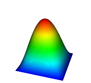
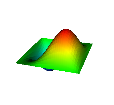
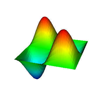
Here, the potential is zero inside the domain, and we know that the eigenvalues are given by \lambda_{(mn)}=\frac{\pi^2}{4}(m^2+n^2) where m,n\in{\mathbb N^+}. Eigenfunctions are sines and cosines with m and n periods in x and y directions. This matches the output our program generates:
These eigenvalues are exactly the ones that correspond to pairs (m,n)=(1,1), (1,2) and (2,1), (2,2), and (3,1). A visualization of the corresponding eigenfunctions would look like this:
 |  |  |
 |  |
It is always worth playing a few games in the playground! So here goes with a few suggestions:
The potential used above (called the infinite well because it is a flat potential surrounded by infinitely high walls) is interesting because it allows for analytically known solutions. Apart from that, it is rather boring, however. That said, it is trivial to play around with the potential by just setting it to something different in the input file. For example, let us assume that we wanted to work with the following potential in 2d:
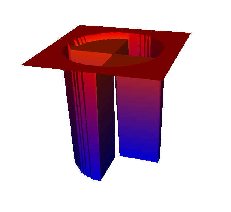
V(x,y) = \left\{ \begin{array}{ll} -100 & \text{if}\ \sqrt{x^2+y^2}<\frac 34 \ \text{and} \ xy>0 \\ -5 & \text{if}\ \sqrt{x^2+y^2}<\frac 34 \ \text{and} \ xy\le 0 \\ 0 & \text{otherwise} \end{array} \right.\quad.
In other words, the potential is -100 in two sectors of a circle of radius 0.75, -5 in the other two sectors, and zero outside the circle. We can achieve this by using the following in the input file :
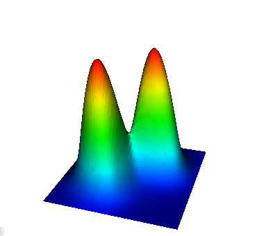
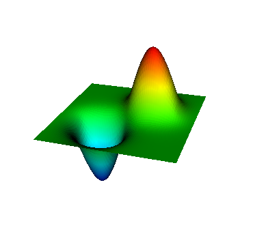
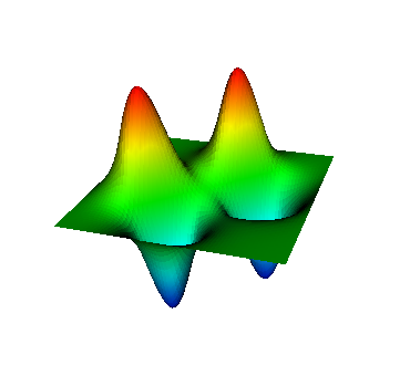
If in addition we also increase the mesh refinement by one level, we get the following results:
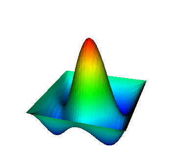
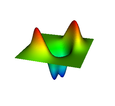
The output file also contains an interpolated version of the potential, which looks like this (note that as expected the lowest few eigenmodes have probability densities |\Psi(\mathbf x)|^2 that are significant only where the potential is the lowest, i.e. in the top right and bottom left sector of inner circle of the potential):
The first five eigenfunctions are now like this:
 |  |  |
 |  |
In our derivation of the problem we have assumed that the particle is confined to a domain \Omega and that at the boundary of this domain its probability |\Psi|^2 of being is zero. This is equivalent to solving the eigenvalue problem on all of {\mathbb R}^d and assuming that the energy potential is finite only inside a region \Omega and infinite outside. It is relatively easy to show that |\Psi(\mathbf x)|^2 at all locations \mathbf x where V(\mathbf x)=\infty. So the question is what happens if our potential is not of this form, i.e. there is no bounded domain outside of which the potential is infinite? In that case, it may be worth to just consider a very large domain at the boundary of which V(\mathbf x) is at least very large, if not infinite. Play around with a few cases like this and explore how the spectrum and eigenfunctions change as we make the computational region larger and larger.
What happens if we investigate the simple harmonic oscillator problem V(\mathbf x)=c|\mathbf x|^2? This potential is exactly of the form discussed in the previous paragraph and has hyper spherical symmetry. One may want to use a large spherical domain with a large outer radius, to approximate the whole-space problem (say, by invoking GridGenerator::hyper_ball).
The plots above show the wave function \Psi(\mathbf x), but the physical quantity of interest is actually the probability density |\Psi(\mathbf x)|^2 for the particle to be at location \mathbf x. Some visualization programs can compute derived quantities from the data in an input file, but we can also do so right away when creating the output file. The facility to do that is the DataPostprocessor class that can be used in conjunction with the DataOut class. Examples of how this can be done can be found in step-29 and step-33.
What happens if the particle in the box has internal degrees of freedom? For example, if the particle were a spin- 1/2 particle? In that case, we may want to start solving a vector-valued problem instead.
Our implementation of the deal.II library here uses the PETScWrappers and SLEPcWrappers and is suitable for running on serial machine architecture. However, for larger grids and with a larger number of degrees-of-freedom, we may want to run our application on parallel architectures. A parallel implementation of the above code can be particularly useful here since the generalized eigenspectrum problem is somewhat more expensive to solve than the standard problems considered in most of the earlier tutorials. Fortunately, modifying the above program to be MPI compliant is a relatively straightforward procedure. A sketch of how this can be done can be found in step-17.
Finally, there are alternatives to using the SLEPc eigenvalue solvers. deal.II has interfaces to one of them, ARPACK (see the ARPACK configuration page for setup instructions), implemented in the ArpackSolver class. Here is a short and quick overview of what one would need to change to use it, provided you have a working installation of ARPACK and deal.II has been configured properly for it (see the deal.II README file):
First, in order to use the ARPACK interfaces, we can go back to using standard deal.II matrices and vectors, so we start by replacing the PETSc and SLEPc headers
with these:
ARPACK allows complex eigenvalues, so we will also need
Secondly, we switch back to the deal.II matrix and vector definitions in the main class:
and initialize them as usual in make_grid_and_dofs():
For solving the eigenvalue problem with ARPACK, we finally need to modify solve():
Note how we have used an exact decomposition (using SparseDirectUMFPACK) as a preconditioner to ARPACK.