This tutorial depends on step-6.
This program was contributed by Manaswinee Bezbaruah (Texas A&M University), and Matthias Maier (Texas A&M University).
Introduction
A surface plasmon-polariton (SPP) is a slowly decaying electromagnetic wave that is confined near a metal-air (or similar) interface. SPP structures on novel "2D" materials such as graphene, a monoatomic layer of carbon atoms arranged in a hexagonal lattice, typically have wavelengths much shorter than the wavelength of the free-space radiation. This scale separation makes SPPs on 2D materials a promising ingredient in the design of novel optical devices.
In the following, we discuss a method for observing SPPs numerically by solving a suitable electromagnetic model based on time-harmonic Maxwell's equations which incorporate jump conditions on lower-dimensional material interfaces: The conducting sheet is modeled as an idealized hypersurface with an effective electric conductivity and the weak discontinuity for the tangential surface appears naturally in the variational form.
This tutorial presents a direct solver for the time-harmonic Maxwell equations for scattering configurations with lower-dimensional interfaces. In particular, we discuss using complex values, simple first-order absorbing boundary conditions, and a more sophisticated perfectly matched layer (PML) boundary condition for electromagnetic waves.
Time-Harmonic Maxwell's Equations with interface conditions
We start the discussion with a short derivation of the governing equations and some literature references.
Derivation of time-harmonic Maxwell's equations
In two ( d=2) or three ( d=3) spatial dimensions, the time evolution of an electromagnetic wave (\mathbf{E},\mathbf{H}) that consists of an electric field component \mathbf{E}(t,\mathbf{x})\;:\;\mathbb{R}\times\mathbb{R}^d\to\mathbb{R}^d and a magnetic field component \mathbf{H}(t,\mathbf{x})\;:\;\mathbb{R}\times\mathbb{R}^d\to\mathbb{R}^d is described by Maxwell's equations [192], [156] :
\begin{align*}
\frac{\partial}{\partial t} \mathbf{H} + \nabla \times \mathbf{E} &= -\mathbf{M}_a,
\\
\nabla \cdot \mathbf{H} &= \rho_m,
\\
\frac{\partial}{\partial t} (\varepsilon\mathbf{E}) - \nabla\times(\mu^{-1}\mathbf{H}) &= - \mathbf{J}_a,
\\
\nabla\cdot(\varepsilon\mathbf{E}) &= \rho.
\end{align*}
Here, \nabla\times is the curl operator, \nabla\cdot is the divergence operator, \varepsilon is the electric permittivity, \mu is the magnetic permeability, \rho is the electric charge density, and \rho_m is a corresponding (hypothetical) magnetic monopole density. \mathbf{J}_a and \mathbf{M}_a are the electric and magnetic flux densities which are related to their respective charge densities by the conservation equations [192]
\frac{\partial}{\partial t} \rho + \nabla\cdot\mathbf{J}_a = 0
\text{ and }
\frac{\partial}{\partial t} \rho_m + \nabla\cdot\mathbf{M}_a = 0.
We now make the important assumption that the material parameters \varepsilon and \mu are time-independent and that the fields \mathbf{E} and \mathbf{H}, the fluxes \mathbf{M}_a and \mathbf{J}_a, as well as the densities \rho and \rho_m are all time-harmonic, i.e., their time evolution is completely described by
\mathbf{F}(\mathbf{x},t) = \text{Re}\{e^{-i\omega
t}\tilde{\mathbf{F}}(\mathbf{x})\},
in which \omega is the temporal angular frequency and \tilde{\mathbf{F}}(\mathbf{x}) is a corresponding complex-valued vector field (or density). Inserting this ansatz into Maxwell's equations, substituting the charge conservation equations and some minor algebra then yields the so-called time-harmonic Maxwell's equations:
\begin{align*}
-i\omega \tilde{\mathbf{H}} + \nabla \times \tilde{\mathbf{E}} &=
-\tilde{\mathbf{M}}_a,
\\
\nabla \cdot \tilde{\mathbf{H}} &= \frac{1}{i\omega}\nabla \cdot
\tilde{\mathbf{M}}_a,
\\
i\omega\varepsilon\tilde{\mathbf{E}} +
\nabla\times(\mu^{-1}\tilde{\mathbf{H}}) &= \tilde{\mathbf{J}}_a,
\\
\nabla\cdot(\varepsilon\tilde{\mathbf{E}}) &=
\frac{1}{i\omega}\nabla\cdot\tilde{\mathbf{J}}_a.
\end{align*}
For the sake of better readability we will now drop the tilde and simply write \mathbf{E}(\mathbf{x}), \mathbf{H}(\mathbf{x}), etc., when referring to the time-harmonic fields.
Jump conditions on lower dimensional interfaces
Graphene is a two-dimensional carbon allotrope with a single atom layer that is arranged in a honeycomb lattice [167]. Due to its atomic thickness it is an example of a so-called 2D material: Compared to the other spatial dimensions (where graphene samples can reach up to several centimeters) the atomistic thickness of graphene typically ranges around 2.5 ångstrom ( 2.5\times10^{-10}\text{m}). We will thus model graphene as a lower-dimensional interface \Sigma embedded into the computational domain \Omega\subset\mathbb{R}^d. More precisely, \Sigma is a two-dimensional sheet in three spatial dimensions, or a one-dimensional line in two spatial dimensions. The special electronic structure of graphene gives rise to a current density on the lower-dimensional interface that is modeled with an effective surface conductivity \sigma^\Sigma obeying Ohm's Law:
\mathbf{J}^\Sigma=\sigma^\Sigma\,\mathbf{E}_T
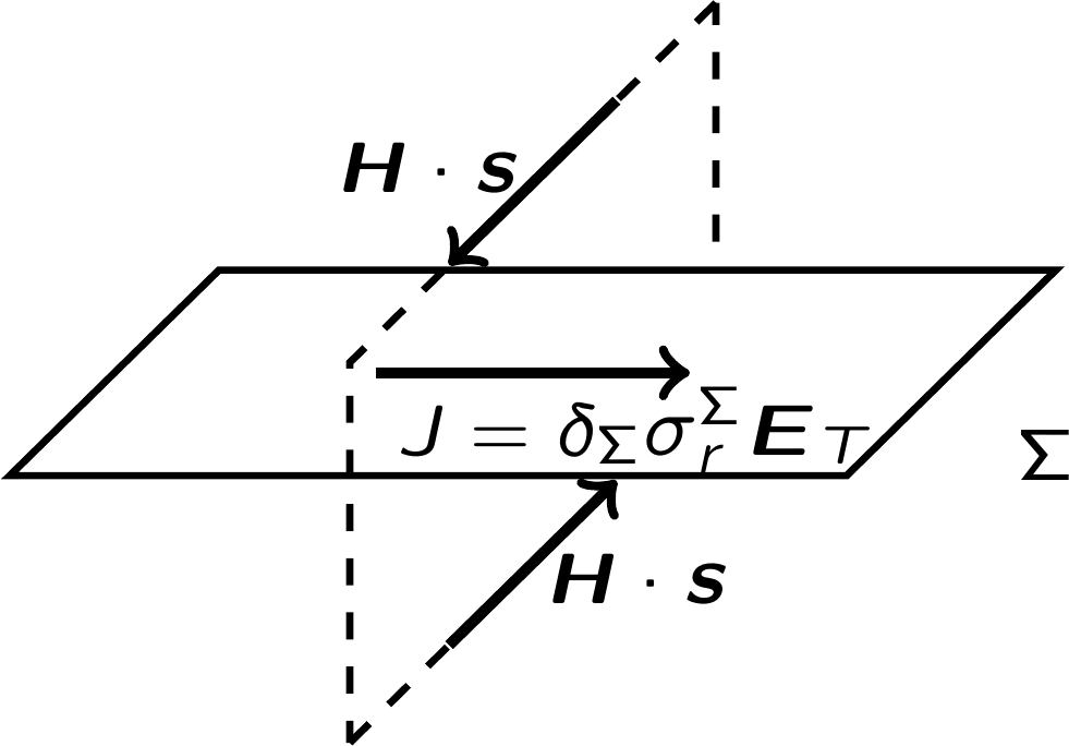
in which \mathbf{J}^\Sigma is the surface current density, \mathbf{E}_T denotes the tangential part of the electric field \mathbf{E}, and \sigma^\Sigma is an appropriately chosen surface conductivity that will be discussed in more detail below. The surface current density gives rise to a jump condition on \Sigma in the tangential component of the magnetic field. This is best seen by visualizing Ampère's law:

and then taking the limit of the upper and lower part of the line integral approaching the sheet. In contrast, the tangential part of the electric field is continuous. By fixing a unit normal \mathbf{\nu} on the hypersurface \Sigma both jump conditions are
\begin{align*}
\mathbf{\nu} \times \left[(\mu^{-1}\mathbf{H})^+ - (\mu^{-1}\mathbf{H})^-\right]|_{\Sigma}
&= \sigma^{\Sigma}\left[(\mathbf{\nu}\times \mathbf{E}\times \mathbf{\nu})\right]|_{\Sigma},
\\
\mathbf{\nu} \times \left[\mathbf{E}^+ - \mathbf{E}^-\right]|_{\Sigma} &= 0.
\end{align*}
The notation \mathbf{F}^\pm indicates the limit values of the field when approaching the interface from above or below the interface: \mathbf{F}^\pm(\mathbf{x})=\lim_{\delta\to0,\delta>0}\mathbf{F}(\mathbf{x}\pm\delta\mathbf{\nu}).
Rescaling
We will be using a rescaled version of the Maxwell's equations described above. The rescaling has the following key differences:
-
Every length is rescaled by the free-space wavelength 2\pi k^{-1}
\dealcoloneq 2\pi(\omega\sqrt{\varepsilon_0\mu_0})^{-1}, in which \varepsilon_0 and \mu_0 denote the vacuum dielectric permittivity and magnetic permeability, respectively.
-
\mathbf{E}, \mathbf{H}, \mathbf{J}_a, \mathbf{M}_a are all rescaled by typical electric current strength J_0, i.e., the strength of the prescribed dipole source at location a in the e_i direction in Cartesian coordinates (here, \delta is the Dirac delta operator).
\mathbf{J}_a = J_0 \mathbf{e}_i\delta(x-a)
Accordingly, our electric permittivity and magnetic permeability are rescaled by \varepsilon_0 and \mu_0 as
\mu_r = \frac{1}{\mu_0}\mu
\text{ and }
\varepsilon_r = \frac{1}{\varepsilon_0}\varepsilon.
We use the free-space wave number k_0 = \omega\sqrt{\varepsilon_0\mu_0} and the dipole strength, J_0 to arrive at the following rescaling of the vector fields and coordinates:
\begin{align*}
\hat{x} = k_0x, &\qquad
\hat{\nabla} = \frac{1}{k_0}\nabla,\\
\hat{\mathbf{H}} = \frac{k_0}{J_0}\mu^{-1}\mathbf{H},&\qquad
\hat{\mathbf{E}} = \frac{k_0^2}{\omega\mu_0 J_0}\mathbf{E},\\
\hat{\mathbf{J}}_a = \frac{1}{J_0}\mathbf{J}_a,&\qquad
\hat{\mathbf{M}}_a = \frac{k_0}{\omega\mu_0 J_0}\mathbf{M}_a.
\end{align*}
Finally, the interface conductivity is rescaled as
\sigma^{\Sigma}_r = \sqrt{\frac{\mu_0}{\varepsilon_0}}\sigma^{\Sigma}.
Accordingly, our rescaled equations are
\begin{align*}
-i\mu_r \hat{\mathbf{H}} + \hat{\nabla} \times \hat{\mathbf{E}}
&= -\hat{\mathbf{M}}_a,
\\
\hat{\nabla} \cdot (\mu_r\hat{\mathbf{H}}) &= \frac{1}{i\omega}\hat{\nabla}
\cdot \hat{\mathbf{M}}_a,
\\
i\varepsilon_r\hat{\mathbf{E}} + \nabla\times(\mu^{-1}\mathbf{H})
&= \mathbf{J}_a,
\\
\nabla\cdot(\varepsilon\mathbf{E}) &= \frac{1}{i\omega}\hat{\nabla}
\cdot\hat{\mathbf{J}}_a.
\end{align*}
We will omit the hat in further discussion for ease of notation.
Variational Statement
Let \Omega \subset \mathbb{R}^n, (n = 2,3) be a simply connected and bounded domain with Lipschitz-continuous and piecewise smooth boundary, \partial\Omega. Let \Sigma be an oriented, Lipschitz-continuous, piecewise smooth hypersurface. Fix a normal field \nu on \Sigma and let n denote the outer normal vector on \partial\Omega.
In order to arrive at the variational form, we will substitute for \mathbf{H} in the first equation and obtain
\nabla \times (\mu_r^{-1}\nabla\times\mathbf{E}) - \varepsilon_r \mathbf{E}
= i\mathbf{J}_a - \nabla\times (\mu_r^{-1}\mathbf{M}_a).
Now, consider a smooth test function \varphi with complex conjugate \bar{\varphi}. Multiply both sides of the above equation by \bar{\varphi} and integrate by parts in \Omega\backslash\Sigma.
\int_\Omega (\mu_r^{-1}\nabla\times\mathbf{E})\cdot (\nabla\times\bar{\varphi})\;\text{d}x
- \int_\Omega \varepsilon_r\mathbf{E} \cdot \bar{\varphi}\;\text{d}x
- \int_\Sigma [\nu \times (\mu_r^{-1}\nabla\times\mathbf{E} +
\mu^{-1}\mathbf{M}_a)]_{\Sigma}\cdot \bar{\varphi}_T\;\text{d}o_x\\
\qquad - \int_{\partial\Omega} (\nu \times (\mu_r^{-1}\nabla\times\mathbf{E} +
\mu^{-1}\mathbf{M}_a)) \cdot \bar{\varphi}_T\;\text{d}o_x =
i\int_\Omega \mathbf{J}_a \cdot \bar{\varphi}\;\text{d}x
- \int_\Omega \mu_r^{-1}\mathbf{M}_a \cdot (\nabla \times \bar{\varphi})\;\text{d}x.
We use the subscript T to denote the tangential part of the given vector and [\cdot]_{\Sigma} to denote a jump over \Sigma, i.e.,
\mathbf{F}_T = (\mathbf{\nu}\times \mathbf{F})\times\mathbf{\nu}
\text{ and }
[\mathbf{F}]_{\Sigma}(\mathbf{x}) = \lim\limits_{s\searrow 0}(\mathbf{F}(\mathbf{x}+s\mathbf{\nu})-\mathbf{F}(\mathbf{x}-s\mathbf{\nu}))
for \mathbf{x}\in \Sigma.
For the computational domain \Omega, we introduce the absorbing boundary condition at \partial\Omega, which is obtained by using a first-order approximation of the Silver-Müller radiation condition, truncated at \partial\Omega [156].
\nu\times\mathbf{H}+\sqrt{\mu_r^{-1}\varepsilon_r}\mathbf{E}=0\qquad x\in\partial\Omega
We assume that \mu_r^{-1} and \varepsilon have well-defined square roots. In our numerical computation, we combine the above absorbing boundary condition with a PML.
The jump condition can be expressed as a weak discontinuity as follows:
[\nu \times (\mu_r^{-1}\nabla\times\mathbf{E} + \mu^{-1}\mathbf{M}_a)]_{\Sigma}
= i\sigma_r^{\Sigma}\mathbf{E}_T,\qquad \text{on }\Sigma\\
\nu \times (\mu_r^{-1}\nabla\times\mathbf{E} + \mu^{-1}\mathbf{M}_a)
= -i\sqrt{\mu_r^{-1}\varepsilon_r}\mathbf{E}_T,\qquad \text{on }\partial\Omega.
Combining, our weak form is as follows:
\int_\Omega (\mu_r^{-1}\nabla\times\mathbf{E})\cdot (\nabla\times\bar{\varphi})\;\text{d}x
- \int_\Omega \varepsilon_r\mathbf{E} \cdot \bar{\varphi}\;\text{d}x
- i\int_\Sigma (\sigma_r^{\Sigma}\mathbf{E}_T) \cdot \bar{\varphi}_T\;\text{d}o_x\\
\qquad - i\int_{\partial\Omega} (\sqrt{\mu_r^{-1}\varepsilon}\mathbf{E}_T) \cdot
(\nabla\times\bar{\varphi}_T)\;\text{d}o_x.=
i\int_\Omega \mathbf{J}_a \cdot \bar{\varphi}\;\text{d}x
- \int_\Omega \mu_r^{-1}\mathbf{M}_a \cdot (\nabla \times \bar{\varphi})\;\text{d}x.
Assume that \sigma_r^{\Sigma} \in L^{\infty}(\Sigma)^{2\times 2} is matrix-valued and symmetric, and has a semidefinite real and complex part. Let \varepsilon_r be a smooth scalar function with -\text{Im}(\varepsilon_r) = 0, or \text{Im}(\varepsilon_r)\ge c > 0 in \Omega. \mu_r^{-1} is a smooth scalar such that \sqrt{\mu_r^{-1}\varepsilon_r} is real valued and strictly positive in \partial\Omega.
\mathbf{H}(\text{curl};\Omega) is space of vector-valued, measurable and square integrable functions whose weak curl admits a representation by a square integrable function. Define a Hilbert space
X(\Omega) = \{\varphi \in \mathbf{H}(\text{curl};\Omega)\;\;:\;\; \varphi_T|_{\Sigma}
\in L^2(\Sigma)^2,\;\varphi_T|_{\partial\Omega} \in L^2(\partial\Omega)^2\}
equipped with the norm
\|\varphi\|^2_X = \|\varphi\|^2_{L^2(\Omega)} +
\|\nabla\times\varphi\|^2_{L^2(\Omega)} + \|\varphi_T\|^2_{L^2(\Sigma)} +
\|\varphi_T\|^2_{L^2(\partial\Omega)}.
Define
A(\mathbf{E},\varphi) \dealcoloneq \int_\Omega (\mu_r^{-1}\nabla\times\mathbf{E})\cdot
(\nabla\times\bar{\varphi})\;\text{d}x
- \int_\Omega \varepsilon_r\mathbf{E} \cdot \bar{\varphi}\;\text{d}x
- i\int_\Sigma (\sigma_r^{\Sigma}\mathbf{E}_T) \cdot \bar{\varphi}_T\;\text{d}o_x
- i\int_{\partial\Omega} (\sqrt{\mu_r^{-1}\varepsilon}\mathbf{E}_T) \cdot
(\nabla\times\bar{\varphi}_T)\;\text{d}o_x.\\
F(\varphi) \dealcoloneq i\int_\Omega \mathbf{J}_a \cdot \bar{\varphi}\;\text{d}x
- \int_\Omega \mu_r^{-1}\mathbf{M}_a \cdot (\nabla \times \bar{\varphi})\;\text{d}x.
Then, our rescaled weak formulation is:
\text{Find a unique } \mathbf{E} \in X(\Omega) \text{ such that, for all } \varphi \in X(\Omega),
A(\mathbf{E},\varphi) = F(\varphi).
Absorbing boundary conditions and the perfectly matched layer
Moreover, the above equations are supplemented by the Silver-Müller radiation condition, if the ambient (unbounded) medium is isotropic. This amounts to the requirement that \mathbf{E} and \mathbf{H} both approach a spherical wave uniformly in the radial direction for points at infinity and away from the conducting sheet, i.e.,
\lim\limits_{|x|\to\infty} \{\mathbf{H}\times x - c^{-1}|x|\mathbf{E}\} = 0
\text{ and }
\lim\limits_{|x|\to\infty} \{\mathbf{E}\times x - c^{-1}|x|\mathbf{H}\} = 0
\text{ for }
x \not\in \Sigma.
In our case, we eliminate reflection from infinity by implementing a PML, which is described at length below, and avoid the explicit use of the last condition.
Discretization Scheme
The variational form is discretized on a non-uniform quadrilateral mesh with higher-order, curl-conforming Nédélec elements implemented by the FE_NedelecSZ class. This way the interface with a weak discontinuity is optimal, and we get optimal convergence rates.
Consider the finite element subspace X_h(\Omega) \subset X(\Omega). Define the matrices
A_{ij} = \int_\Omega (\mu_r^{-1}\nabla \times \varphi_j) \cdot
(\nabla\times\bar{\varphi}_i)\;\text{d}x
- \int_\Omega \varepsilon_r\varphi_j \cdot \bar{\varphi}_i\;\text{d}x
- i\int_\Sigma (\sigma_r^{\Sigma}\varphi_{j_T}) \cdot
\bar{\varphi}_{i_T}\;\text{d}o_x
- i\int_{\partial\Omega} (\sqrt{\mu_r^{-1}\varepsilon}\varphi_{j_T})
\cdot (\nabla\times \bar{\varphi}_{i_T})\;\text{d}o_x,
F_i = i\int_\Omega \mathbf{J}_a \cdot \bar{\varphi_i}\;\text{d}x
- \int_\Omega \mu_r^{-1}\mathbf{M}_a \cdot (\nabla \times \bar{\varphi_i})
\;\text{d}x.
Then under the assumption of a sufficiently refined initial mesh the discretized variational problem is:
\text{Find a unique } \mathbf{E}_h = \sum_j U_j\mathbf{\varphi}_j \in
X_h(\Omega) \text{ such that}
\sum_jA_{ij}U_j = F_i\qquad\text{for all }i.
Perfectly Matched Layer
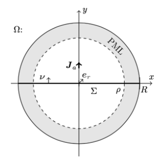
The SPP amplitude is negatively affected by the absorbing boundary condition and this causes the solution image to be distorted. In order to reduce the resonance and distortion in our solutions, we are implementing a Perfectly Matched Layer (PML) in the scattering configuration.
The concept of a PML was pioneered by Bérenger [28] and it is is an indispensable tool for truncating unbounded domains for wave equations and often used in the numerical approximation of scattering problems. It is essentially a thin layer with modified material parameters placed near the boundary such that all outgoing electromagnetic waves decay exponentially with no “artificial” reflection due to truncation of the domain.
Our PML is a concentric circle with modified material coefficients ( \varepsilon_r, \mu_r, \sigma). It is located in a small region near the boundary \partial\Omega and the transformation of the material coordinates is chosen to be a function of the radial distance \rho from the origin e_r. The normal field \nu of \Sigma is orthogonal to the radial direction e_r, which makes \mathbf{J}_a \equiv 0 and \mathbf{M}_a \equiv 0 within the PML.

Introduce a change of coordinates
x \to \bar{x} =
\begin{cases}
x + ie_r\int\limits_\rho^r s(\tau)\text{d}\tau,\;\;\;\;\;\;\; r\ge\rho\\
x\;\;\;\;\;\;\;\;\;\text{otherwise}
\end{cases}
in which r = e_r \cdot x and s(\tau) is an appropriately chosen, nonnegative scaling function.
We introduce the following 2\times2 matrices
\begin{align*}
A &= T_{e_xe_r}^{-1} \text{diag}\left(\frac{1}{\bar{d}^2},
\frac{1}{d\bar{d}}\right)T_{e_xe_r}
\\
B &= T_{e_xe_r}^{-1} \text{diag}\left(d,\bar{d}\right)T_{e_xe_r}
\\
C &= T_{e_xe_r}^{-1} \text{diag}\left(\frac{1}{\bar{d}},\frac{1}{d}\right)
T_{e_xe_r}
\end{align*}
in which
\begin{align*}
d &= 1 + is(r) \\
\bar{d} &= 1 + i/r \int\limits_{\rho}^{r}s(\tau)\text{d}\tau
\end{align*}
and T_{e_xe_r} is the rotation matrix which rotates e_r onto e_x. Thus, after applying the rescaling, we get the following modified parameters
\begin{align*}
\bar{\mu}_r^{-1} &= \frac{\mu_r^{-1}}{d},
\\
\bar{\varepsilon}_r &= A^{-1} \varepsilon_r B^{-1}, \text{ and }
\\
\bar{\sigma}^{\Sigma}_r &= C^{-1} \sigma^{\Sigma}_r B^{-1}.
\end{align*}
These PML transformations are implemented in our PerfectlyMatchedLayer class. After the PML is implemented, the electromagnetic wave essentially decays exponentially within the PML region near the boundary, therefore reducing reflection from the boundary of our finite domain. The decay function also depends on the strength of our PML, which can be adjusted to see more or less visible decaying in the PML region.
The commented program
Include files
The set of include files is quite standard. The most notable include is the fe/fe_nedelec_sz.h file which allows us to use the FE_NedelecSZ elements. This is an implementation of the H^{curl} conforming Nédélec Elements that resolves the sign conflict issues that arise from parametrization (for details we refer to the documentation of the FE_NedelecSZ element).
#include <deal.II/base/function.h>
#include <deal.II/base/parameter_acceptor.h>
#include <deal.II/base/quadrature_lib.h>
#include <deal.II/base/tensor.h>
#include <deal.II/dofs/dof_accessor.h>
#include <deal.II/dofs/dof_handler.h>
#include <deal.II/dofs/dof_renumbering.h>
#include <deal.II/dofs/dof_tools.h>
#include <deal.II/fe/fe_nedelec_sz.h>
#include <deal.II/fe/fe_q.h>
#include <deal.II/fe/fe_system.h>
#include <deal.II/fe/fe_values.h>
#include <deal.II/grid/grid_generator.h>
#include <deal.II/grid/grid_refinement.h>
#include <deal.II/grid/tria.h>
#include <deal.II/grid/tria_accessor.h>
#include <deal.II/grid/tria_iterator.h>
#include <deal.II/lac/affine_constraints.h>
#include <deal.II/lac/dynamic_sparsity_pattern.h>
#include <deal.II/lac/full_matrix.h>
#include <deal.II/lac/precondition.h>
#include <deal.II/lac/solver_cg.h>
#include <deal.II/lac/sparse_direct.h>
#include <deal.II/lac/sparse_ilu.h>
#include <deal.II/lac/sparse_matrix.h>
#include <deal.II/lac/vector.h>
#include <deal.II/numerics/data_out.h>
#include <deal.II/numerics/error_estimator.h>
#include <deal.II/numerics/vector_tools.h>
#include <fstream>
#include <iostream>
#include <memory>
Class Template Declarations
We begin our actual implementation by declaring all classes with their data structures and methods upfront.
namespace Step81
{
using namespace std::complex_literals;
Parameters Class
The Parameters class inherits ParameterAcceptor, and instantiates all the coefficients in our variational equations. These coefficients are passed through ParameterAcceptor and are editable through a .prm file. More explanation on the use and inheritance from the ParameterAcceptor can be found in step-60.
epsilon is the Electric Permittivity coefficient and it is a rank 2 tensor. Depending on the material, we assign the i^th diagonal element of the tensor to the material epsilon value (one of the private epsilon_1_ or epsilon_2_ variables).
mu_inv is the inverse of the Magnetic Permiability coefficient and it is a complex number.
sigma is the Surface Conductivity coefficient between material left and material right and it is a rank 2 tensor. It is only changed if we are at the interface between two materials. If we are at an interface, we assign the i^th diagonal element of the tensor to the private sigma_ value.
J_a is the strength and orientation of the dipole. As mentioned in the rescaling,
\mathbf{J}_a = J_0 \mathbf{e}_i\delta(x-a)
It is a rank 1 tensor that depends on the private dipole_position, dipole_radius, dipole_strength, dipole_orientation variables.
template <int dim>
{
public:
Parameters();
using rank0_type = std::complex<double>;
public:
private:
rank2_type epsilon_1;
rank2_type epsilon_2;
std::complex<double> mu_inv_1;
std::complex<double> mu_inv_2;
rank2_type sigma_tensor;
double dipole_radius;
rank0_type dipole_strength;
};
template <int dim>
Parameters<dim>::Parameters()
{
epsilon_1[0][0] = 1.;
epsilon_1[1][1] = 1.;
add_parameter("material 1 epsilon",
epsilon_1,
"relative permittivity of material 1");
epsilon_2[0][0] = 1.;
epsilon_2[1][1] = 1.;
add_parameter("material 2 epsilon",
epsilon_2,
"relative permittivity of material 2");
mu_inv_1 = 1.;
add_parameter("material 1 mu_inv",
mu_inv_1,
"inverse of relative permeability of material 1");
mu_inv_2 = 1.;
add_parameter("material 2 mu_inv",
mu_inv_2,
"inverse of relative permeability of material 2");
sigma_tensor[0][0] = std::complex<double>(0.001, 0.2);
sigma_tensor[1][1] = std::complex<double>(0.001, 0.2);
add_parameter("sigma",
sigma_tensor,
"surface conductivity between material 1 and material 2");
dipole_radius = 0.3;
add_parameter("dipole radius", dipole_radius, "radius of the dipole");
add_parameter("dipole position", dipole_position, "position of the dipole");
add_parameter("dipole orientation",
dipole_orientation,
"orientation of the dipole");
dipole_strength = 1.;
add_parameter("dipole strength", dipole_strength, "strength of the dipole");
}
template <int dim>
typename Parameters<dim>::rank2_type
{
return (material == 1 ? epsilon_1 : epsilon_2);
}
template <int dim>
std::complex<double> Parameters<dim>::mu_inv(
const Point<dim> & ,
{
return (material == 1 ? mu_inv_1 : mu_inv_2);
}
template <int dim>
typename Parameters<dim>::rank2_type
{
return (left == right ? rank2_type() : sigma_tensor);
}
template <int dim>
typename Parameters<dim>::rank1_type
{
rank1_type J_a;
const auto distance = (dipole_position -
point).
norm() / dipole_radius;
if (distance > 1.)
return J_a;
std::cos(distance * M_PI / 2.) / (M_PI / 2. - 2. / M_PI) /
dipole_radius / dipole_radius;
J_a = dipole_strength * dipole_orientation *
scale;
return J_a;
}
double norm(const FEValuesBase< dim > &fe, const ArrayView< const std::vector< Tensor< 1, dim > > > &Du)
Point< spacedim > point(const gp_Pnt &p, const double tolerance=1e-10)
::VectorizedArray< Number, width > cos(const ::VectorizedArray< Number, width > &)
PerfectlyMatchedLayer Class
The PerfectlyMatchedLayer class inherits ParameterAcceptor as well. It implements the transformation matrices used to modify the permittivity and permeability tensors supplied from the Parameters class. The actual transformation of the material tensors will be done in the assembly loop. The radii and the strength of the PML is specified, and the coefficients will be modified using transformation matrices within the PML region. The radii and strength of the PML are editable through a .prm file. The rotation function T_{exer} is the same as introduced in the perfectly matched layer section of the introduction. Similarly, the matrices A, B and C are defined as follows
A = T_{e_xe_r}^{-1}
\text{diag}\left(\frac{1}{\bar{d}^2},\frac{1}{d\bar{d}}\right)T_{e_xe_r},\qquad
B = T_{e_xe_r}^{-1} \text{diag}\left(d,\bar{d}\right)T_{e_xe_r},\qquad
C = T_{e_xe_r}^{-1} \text{diag}\left(\frac{1}{\bar{d}},\frac{1}{d}\right)
T_{e_xe_r}.\qquad
template <int dim>
{
public:
static_assert(dim == 2,
"The perfectly matched layer is only implemented in 2d.");
Parameters<dim> parameters;
PerfectlyMatchedLayer();
std::complex<double> d_bar(
const Point<dim> point);
rank2_type rotation(std::complex<double> d_1,
std::complex<double> d_2,
private:
double inner_radius;
double outer_radius;
double strength;
};
template <int dim>
PerfectlyMatchedLayer<dim>::PerfectlyMatchedLayer()
{
inner_radius = 12.;
add_parameter("inner radius",
inner_radius,
"inner radius of the PML shell");
outer_radius = 20.;
add_parameter("outer radius",
outer_radius,
"outer radius of the PML shell");
strength = 8.;
add_parameter("strength", strength, "strength of the PML");
}
template <int dim>
typename std::complex<double>
PerfectlyMatchedLayer<dim>::d(
const Point<dim> point)
{
if (radius > inner_radius)
{
const double s =
strength * ((radius - inner_radius) * (radius - inner_radius)) /
((outer_radius - inner_radius) * (outer_radius - inner_radius));
return {1.0, s};
}
else
{
return 1.0;
}
}
template <int dim>
typename std::complex<double>
PerfectlyMatchedLayer<dim>::d_bar(
const Point<dim> point)
{
if (radius > inner_radius)
{
const double s_bar =
strength / 3. *
((radius - inner_radius) * (radius - inner_radius) *
(radius - inner_radius)) /
(radius * (outer_radius - inner_radius) *
(outer_radius - inner_radius));
return {1.0, s_bar};
}
else
{
return 1.0;
}
}
template <int dim>
typename PerfectlyMatchedLayer<dim>::rank2_type
PerfectlyMatchedLayer<dim>::rotation(std::complex<double> d_1,
std::complex<double> d_2,
{
rank2_type result;
return result;
}
template <int dim>
typename PerfectlyMatchedLayer<dim>::rank2_type
PerfectlyMatchedLayer<dim>::a_matrix(
const Point<dim> point)
{
const auto d = this->d(point);
const auto d_bar = this->d_bar(point);
return invert(rotation(d * d, d * d_bar, point)) *
rotation(d * d, d * d_bar, point);
}
template <int dim>
typename PerfectlyMatchedLayer<dim>::rank2_type
PerfectlyMatchedLayer<dim>::b_matrix(
const Point<dim> point)
{
const auto d = this->d(point);
const auto d_bar = this->d_bar(point);
return invert(rotation(d, d_bar, point)) * rotation(d, d_bar, point);
}
template <int dim>
typename PerfectlyMatchedLayer<dim>::rank2_type
PerfectlyMatchedLayer<dim>::c_matrix(
const Point<dim> point)
{
const auto d = this->d(point);
const auto d_bar = this->d_bar(point);
return invert(rotation(1. / d_bar, 1. / d, point)) *
rotation(1. / d_bar, 1. / d, point);
}
numbers::NumberTraits< Number >::real_type norm() const
SymmetricTensor< 2, dim, Number > d(const Tensor< 2, dim, Number > &F, const Tensor< 2, dim, Number > &dF_dt)
DEAL_II_HOST constexpr SymmetricTensor< 2, dim, Number > invert(const SymmetricTensor< 2, dim, Number > &)
Maxwell Class
At this point we are ready to declare all the major building blocks of the finite element program which consists of the usual setup and assembly routines. Most of the structure has already been introduced in previous tutorial programs. The Maxwell class also holds private instances of the Parameters and PerfectlyMatchedLayers classes introduced above. The default values of these parameters are set to show us a standing wave with absorbing boundary conditions and a PML.
template <int dim>
{
public:
Maxwell();
void run();
private:
double scaling;
unsigned int refinements;
unsigned int fe_order;
unsigned int quadrature_order;
bool absorbing_boundary;
void parse_parameters_callback();
void make_grid();
void setup_system();
void assemble_system();
void solve();
void output_results();
Parameters<dim> parameters;
PerfectlyMatchedLayer<dim> perfectly_matched_layer;
std::unique_ptr<FiniteElement<dim>> fe;
};
const ::parallel::distributed::Triangulation< dim, spacedim > * triangulation
Class Template Definitions and Implementation
The Constructor
The Constructor simply consists of default initialization a number of discretization parameters (such as the domain size, mesh refinement, and the order of finite elements and quadrature) and declaring a corresponding entry via ParameterAcceptor::add_parameter(). All of these can be modified by editing the .prm file. Absorbing boundary conditions can be controlled with the absorbing_boundary boolean. If absorbing boundary conditions are disabled we simply enforce homogeneous Dirichlet conditions on the tangential component of the electric field. In the context of time-harmonic Maxwell's equations these are also known as perfectly conducting boundary conditions.
template <int dim>
Maxwell<dim>::Maxwell()
{
[&]() { parse_parameters_callback(); });
scaling = 20;
add_parameter("scaling", scaling, "scale of the hypercube geometry");
refinements = 8;
add_parameter("refinements",
refinements,
"number of refinements of the geometry");
fe_order = 0;
add_parameter("fe order", fe_order, "order of the finite element space");
quadrature_order = 1;
add_parameter("quadrature order",
quadrature_order,
"order of the quadrature");
absorbing_boundary = true;
add_parameter("absorbing boundary condition",
absorbing_boundary,
"use absorbing boundary conditions?");
}
template <int dim>
void Maxwell<dim>::parse_parameters_callback()
{
}
boost::signals2::signal< void()> parse_parameters_call_back
The Maxwell::make_grid() routine creates the mesh for the computational domain which in our case is a scaled square domain. Additionally, a material interface is introduced by setting the material id of the upper half ( y>0) to 1 and of the lower half ( y<0) of the computational domain to 2. We are using a block decomposition into real and imaginary matrices for the solution matrices. More details on this are available under the Results section.
template <int dim>
void Maxwell<dim>::make_grid()
{
if (!absorbing_boundary)
{
if (face->at_boundary())
face->set_boundary_id(1);
};
cell->set_material_id(1);
else
cell->set_material_id(2);
<< std::endl;
}
unsigned int n_active_cells() const
void refine_global(const unsigned int times=1)
void hyper_cube(Triangulation< dim, spacedim > &tria, const double left=0., const double right=1., const bool colorize=false)
The Maxwell::setup_system() routine follows the usual routine of enumerating all the degrees of freedom and setting up the matrix and vector objects to hold the system data. Enumerating is done by using DoFHandler::distribute_dofs().
template <int dim>
void Maxwell<dim>::setup_system()
{
dof_handler.distribute_dofs(*fe);
std::cout << "Number of degrees of freedom: " << dof_handler.n_dofs()
<< std::endl;
solution.reinit(dof_handler.n_dofs());
system_rhs.reinit(dof_handler.n_dofs());
constraints.clear();
dof_handler,
0,
0,
constraints);
dof_handler,
dim,
0,
constraints);
constraints.close();
dsp,
constraints,
true);
sparsity_pattern.copy_from(dsp);
system_matrix.reinit(sparsity_pattern);
}
void project_boundary_values_curl_conforming_l2(const DoFHandler< dim, dim > &dof_handler, const unsigned int first_vector_component, const Function< dim, number > &boundary_function, const types::boundary_id boundary_component, AffineConstraints< number > &constraints, const Mapping< dim > &mapping)
void make_hanging_node_constraints(const DoFHandler< dim, spacedim > &dof_handler, AffineConstraints< number > &constraints)
void make_sparsity_pattern(const DoFHandler< dim, spacedim > &dof_handler, SparsityPatternBase &sparsity_pattern, const AffineConstraints< number > &constraints={}, const bool keep_constrained_dofs=true, const types::subdomain_id subdomain_id=numbers::invalid_subdomain_id)
This is a helper function that takes the tangential component of a tensor.
template <int dim>
tangential_part(
const Tensor<1, dim, std::complex<double>> &tensor,
{
auto result = tensor;
result[0] = normal[1] * (tensor[0] * normal[1] - tensor[1] * normal[0]);
result[1] = -normal[0] * (tensor[0] * normal[1] - tensor[1] * normal[0]);
return result;
}
#define DEAL_II_ALWAYS_INLINE
Assemble the stiffness matrix and the right-hand side:
\begin{align*}
A_{ij} = \int_\Omega (\mu_r^{-1}\nabla \times \varphi_j) \cdot
(\nabla\times\bar{\varphi}_i)\text{d}x
- \int_\Omega \varepsilon_r\varphi_j \cdot \bar{\varphi}_i\text{d}x
- i\int_\Sigma (\sigma_r^{\Sigma}(\varphi_j)_T) \cdot
(\bar{\varphi}_i)_T\text{do}x
- i\int_{\partial\Omega} (\sqrt{\mu_r^{-1}\varepsilon}(\varphi_j)_T) \cdot
(\nabla\times(\bar{\varphi}_i)_T)\text{d}x, \end{align*}
\begin{align}
F_i = i\int_\Omega J_a \cdot \bar{\varphi_i}\text{d}x - \int_\Omega
\mu_r^{-1} \cdot (\nabla \times \bar{\varphi_i}) \text{d}x.
\end{align}
In addition, we will be modifying the coefficients if the position of the cell is within the PML region.
template <int dim>
void Maxwell<dim>::assemble_system()
{
const QGauss<dim> quadrature_formula(quadrature_order);
const QGauss<dim - 1> face_quadrature_formula(quadrature_order);
quadrature_formula,
face_quadrature_formula,
const unsigned int dofs_per_cell = fe->dofs_per_cell;
const unsigned int n_q_points = quadrature_formula.size();
const unsigned int n_face_q_points = face_quadrature_formula.size();
std::vector<types::global_dof_index> local_dof_indices(dofs_per_cell);
@ update_values
Shape function values.
@ update_normal_vectors
Normal vectors.
@ update_JxW_values
Transformed quadrature weights.
@ update_gradients
Shape function gradients.
@ update_quadrature_points
Transformed quadrature points.
Next, let us assemble on the interior of the domain on the left hand side. So we are computing
\begin{align*}
\int_\Omega (\mu_r^{-1}\nabla \times \varphi_i) \cdot
(\nabla\times\bar{\varphi}_j)\text{d}x
-
\int_\Omega \varepsilon_r\varphi_i \cdot \bar{\varphi}_j\text{d}x
\end{align*}
and
\begin{align}
i\int_\Omega J_a \cdot \bar{\varphi_i}\text{d}x
- \int_\Omega \mu_r^{-1} \cdot (\nabla \times \bar{\varphi_i})
\text{d}x.
\end{align}
In doing so, we need test functions \varphi_i and \varphi_j, and the curl of these test variables. We must be careful with the signs of the imaginary parts of these complex test variables. Moreover, we have a conditional that changes the parameters if the cell is in the PML region.
for (const auto &cell : dof_handler.active_cell_iterators())
{
fe_values.reinit(cell);
cell_matrix = 0.;
cell_rhs = 0.;
cell->get_dof_indices(local_dof_indices);
const auto id = cell->material_id();
const auto &quadrature_points = fe_values.get_quadrature_points();
for (unsigned int q_point = 0; q_point < n_q_points; ++q_point)
{
const Point<dim> &position = quadrature_points[q_point];
auto mu_inv = parameters.mu_inv(position, id);
auto epsilon = parameters.epsilon(position, id);
const auto J_a = parameters.J_a(position, id);
const auto A = perfectly_matched_layer.a_matrix(position);
const auto B = perfectly_matched_layer.b_matrix(position);
const auto d = perfectly_matched_layer.d(position);
mu_inv = mu_inv / d;
for (const auto i : fe_values.dof_indices())
{
constexpr
std::complex<double> imag{0., 1.};
const auto phi_i =
fe_values[real_part].value(i, q_point) -
imag * fe_values[imag_part].value(i, q_point);
const auto curl_phi_i =
fe_values[real_part].curl(i, q_point) -
imag * fe_values[imag_part].curl(i, q_point);
const auto rhs_value =
(imag * scalar_product(J_a, phi_i)) * fe_values.JxW(q_point);
cell_rhs(i) += rhs_value.real();
for (const auto j : fe_values.dof_indices())
{
const auto phi_j =
fe_values[real_part].value(j, q_point) +
imag * fe_values[imag_part].value(j, q_point);
const auto curl_phi_j =
fe_values[real_part].curl(j, q_point) +
imag * fe_values[imag_part].curl(j, q_point);
const auto temp =
(scalar_product(mu_inv * curl_phi_j, curl_phi_i) -
scalar_product(epsilon * phi_j, phi_i)) *
fe_values.JxW(q_point);
cell_matrix(i, j) += temp.real();
}
}
}
Now we assemble the face and the boundary. The following loops will assemble
\begin{align*}
- i\int_\Sigma (\sigma_r^{\Sigma}(\varphi_i)_T) \cdot
(\bar{\varphi}_j)_T\text{do}x \end{align*}
and
\begin{align}
- i\int_{\partial\Omega} (\sqrt{\mu_r^{-1}\varepsilon}(\varphi_i)_T)
\cdot (\nabla\times(\bar{\varphi}_j)_T)\text{d}x,
\end{align}
respectively. The test variables and the PML are implemented similarly as the domain.
for (const auto &face : cell->face_iterators())
{
if (face->at_boundary())
{
const auto id = face->boundary_id();
if (id != 0)
{
fe_face_values.reinit(cell, face);
for (unsigned int q_point = 0; q_point < n_face_q_points;
++q_point)
{
const auto &position = quadrature_points[q_point];
auto mu_inv = parameters.mu_inv(position, id);
auto epsilon = parameters.epsilon(position, id);
const auto A =
perfectly_matched_layer.a_matrix(position);
const auto B =
perfectly_matched_layer.b_matrix(position);
const auto d = perfectly_matched_layer.d(position);
mu_inv = mu_inv / d;
const auto normal =
fe_face_values.normal_vector(q_point);
for (const auto i : fe_face_values.dof_indices())
{
constexpr
std::complex<double> imag{0., 1.};
const auto phi_i =
fe_face_values[real_part].value(i, q_point) -
imag *
fe_face_values[imag_part].value(i, q_point);
const auto phi_i_T = tangential_part(phi_i, normal);
for (const auto j : fe_face_values.dof_indices())
{
const auto phi_j =
fe_face_values[real_part].value(j, q_point) +
imag *
fe_face_values[imag_part].value(j, q_point);
const auto phi_j_T =
tangential_part(phi_j, normal) *
fe_face_values.JxW(q_point);
const auto prod = mu_inv * epsilon;
const auto sqrt_prod = prod;
const auto temp =
-imag * scalar_product((sqrt_prod * phi_j_T),
phi_i_T);
cell_matrix(i, j) += temp.real();
}
}
}
}
}
else
{
We are on an interior face:
const auto face_index = cell->face_iterator_to_index(face);
const auto id1 = cell->material_id();
const auto id2 = cell->neighbor(face_index)->material_id();
if (id1 == id2)
continue;
fe_face_values.reinit(cell, face);
for (unsigned int q_point = 0; q_point < n_face_q_points;
++q_point)
{
const auto &position = quadrature_points[q_point];
auto sigma = parameters.sigma(position, id1, id2);
const auto B = perfectly_matched_layer.b_matrix(position);
const auto C = perfectly_matched_layer.c_matrix(position);
const auto normal = fe_face_values.normal_vector(q_point);
for (const auto i : fe_face_values.dof_indices())
{
constexpr
std::complex<double> imag{0., 1.};
const auto phi_i =
fe_face_values[real_part].value(i, q_point) -
imag * fe_face_values[imag_part].value(i, q_point);
const auto phi_i_T = tangential_part(phi_i, normal);
for (const auto j : fe_face_values.dof_indices())
{
const auto phi_j =
fe_face_values[real_part].value(j, q_point) +
imag *
fe_face_values[imag_part].value(j, q_point);
const auto phi_j_T = tangential_part(phi_j, normal);
const auto temp =
-imag *
scalar_product((sigma * phi_j_T), phi_i_T) *
fe_face_values.JxW(q_point);
cell_matrix(i, j) += temp.real();
}
}
}
}
}
constraints.distribute_local_to_global(
cell_matrix, cell_rhs, local_dof_indices, system_matrix, system_rhs);
}
}
We use a direct solver from the SparseDirectUMFPACK to solve the system
template <int dim>
void Maxwell<dim>::solve()
{
A_direct.vmult(solution, system_rhs);
}
void initialize(const SparsityPattern &sparsity_pattern)
The output is written into a vtk file with 4 components
template <int dim>
void Maxwell<dim>::output_results()
{
data_out.add_data_vector(solution,
{"real_Ex", "real_Ey", "imag_Ex", "imag_Ey"});
data_out.build_patches();
std::ofstream output("solution.vtk");
data_out.write_vtk(output);
}
template <int dim>
void Maxwell<dim>::run()
{
make_grid();
setup_system();
assemble_system();
solve();
output_results();
}
}
void attach_dof_handler(const DoFHandler< dim, spacedim > &)
The following main function calls the class step-81(), initializes the ParameterAcceptor, and calls the run() function.
int main()
{
try
{
Step81::Maxwell<2> maxwell_2d;
maxwell_2d.run();
}
catch (std::exception &exc)
{
std::cerr << std::endl
<< std::endl
<< "----------------------------------------------------"
<< std::endl;
std::cerr << "Exception on processing: " << std::endl
<< exc.what() << std::endl
<< "Aborting!" << std::endl
<< "----------------------------------------------------"
<< std::endl;
return 1;
}
catch (...)
{
std::cerr << std::endl
<< std::endl
<< "----------------------------------------------------"
<< std::endl;
std::cerr << "Unknown exception!" << std::endl
<< "Aborting!" << std::endl
<< "----------------------------------------------------"
<< std::endl;
return 1;
}
return 0;
}
static void initialize(const std::string &filename="", const std::string &output_filename="", const ParameterHandler::OutputStyle output_style_for_output_filename=ParameterHandler::Short, ParameterHandler &prm=ParameterAcceptor::prm, const ParameterHandler::OutputStyle output_style_for_filename=ParameterHandler::DefaultStyle)
Results
The solution is written to a .vtk file with four components. These are the real and imaginary parts of the E_x and E_y solution waves. With the current setup, the output should read
Number of active cells: 4096
Number of degrees of freedom: 16640
Program ended with exit code: 0
Absorbing boundary conditions and the PML
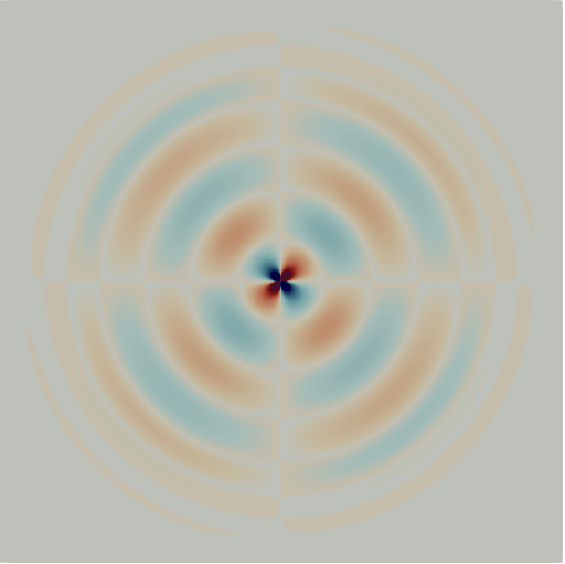
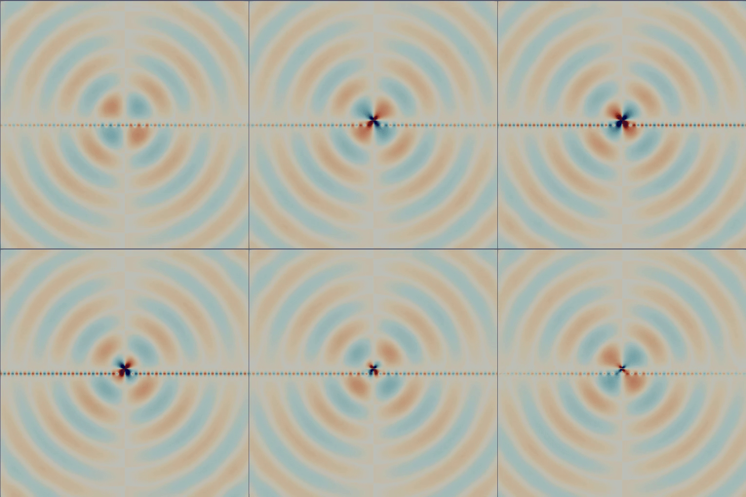
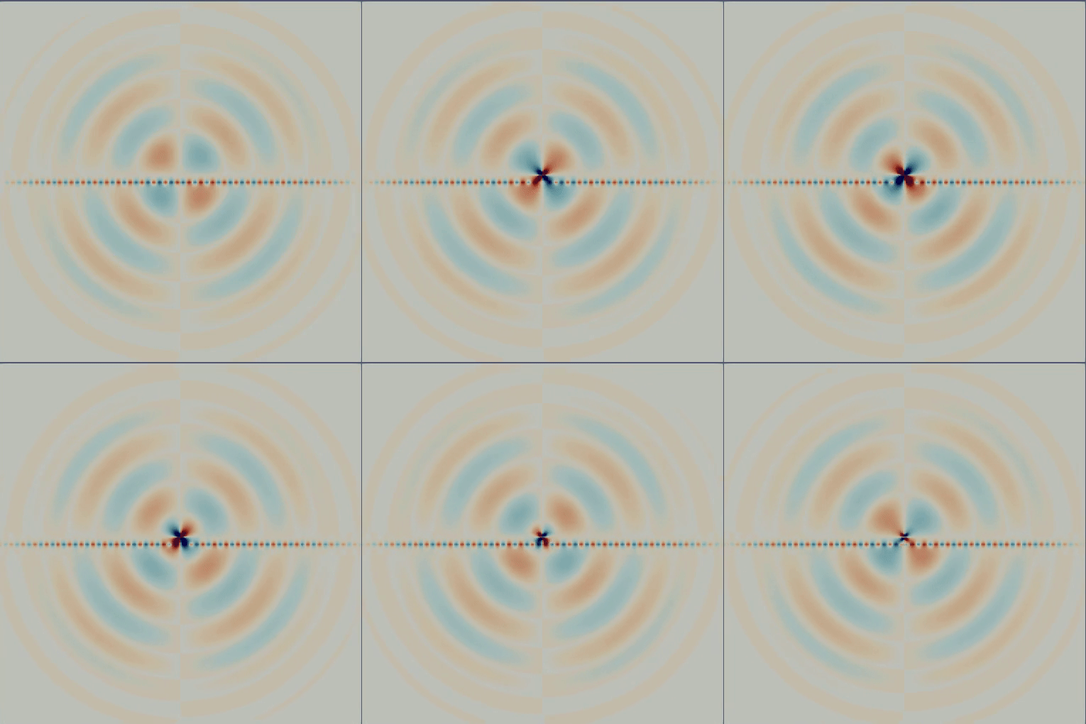
The following images are the outputs for the imaginary E_x without the interface and with the dipole centered at (0,0). In order to remove the interface, the surface conductivity is set to 0. First, we turn off the absorbing boundary conditions and the PML. Second, we want to see the effect of the PML when absorbing boundary conditions apply. So we set absorbing boundary conditions to true and leave the PML strength to 0. Lastly, we increase the strength of the PML to 4. Change the following in the .prm file :
# use absorbing boundary conditions?
set absorbing boundary condition = false
# position of the dipole
set dipole position = 0, 0
# strength of the PML
set strength = 0
# surface conductivity between material 1 and material 2
set sigma = 0, 0; 0, 0| 0, 0; 0, 0
Following are the output images:
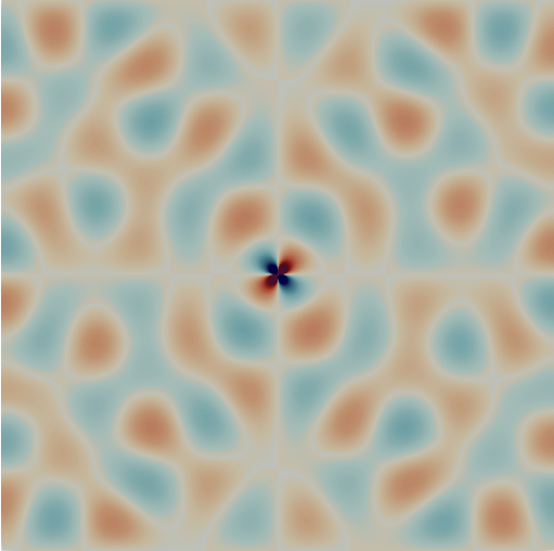
Solution with no interface, Dirichlet boundary conditions and PML strength 0.
| | 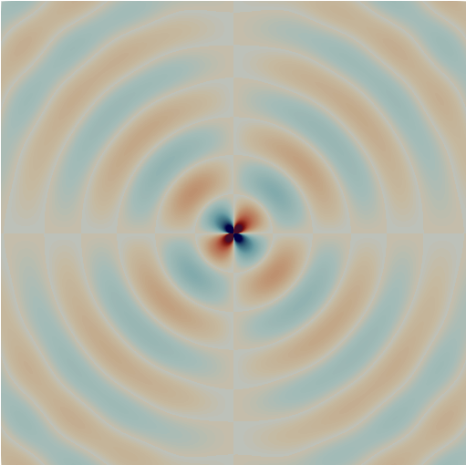
Solution with no interface, absorbing boundary conditions and PML strength 0.
| | 
Solution with no interface, absorbing boundary conditions and PML strength 4.
|
We observe that with absorbing boundary conditions and in absence of the PML, there is a lot of distortion and resonance (the real parts will not be generated without a PML). This is, as we stipulated, due to reflection from infinity. As we see, a much more coherent image is generated with an appropriate PML.
Surface Plasmon Polariton
Now, let's generate a standing wave by adding an interface at the center. In order to observe this effect, we offset the center of the dipole to (0,
0.8) and set the surface conductivity back to (0.001, 0.2):
# position of the dipole
set dipole position = 0, 0.8
# surface conductivity between material 1 and material 2
set sigma = 0.001, 0.2; 0, 0| 0, 0; 0.001, 0.2
Once again, we will visualize the output with absorbing boundary conditions and PML strength 0 and with absorbing boundary conditions and PML strength
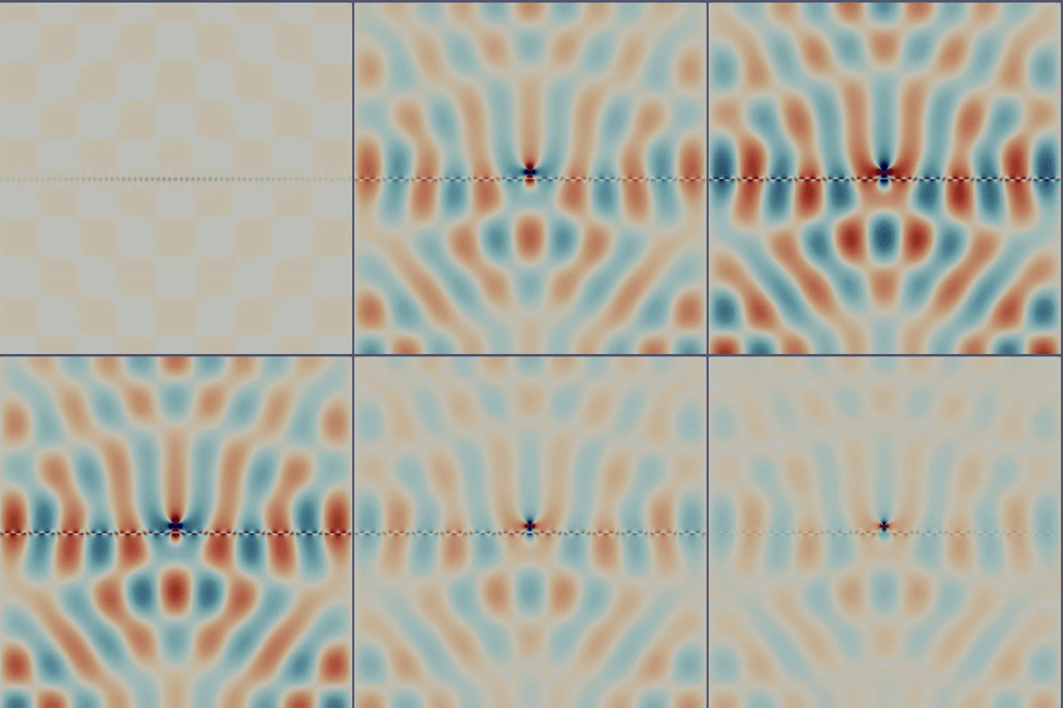
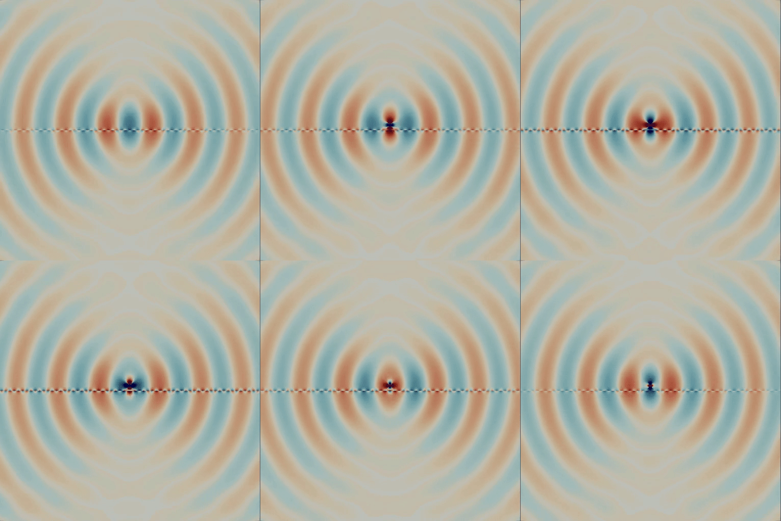
- The following tables are the imaginary part of E_x and the real part of E_x.
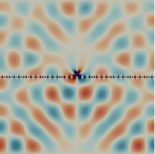
Solution with an interface, Dirichlet boundary conditions and PML strength 0.
| | 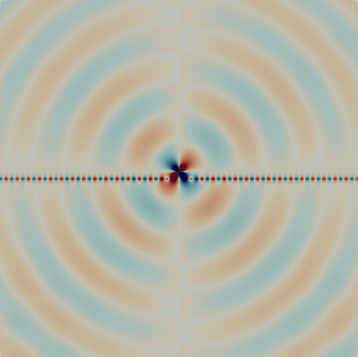
Solution with an interface, absorbing boundary conditions and PML strength 0.
| | 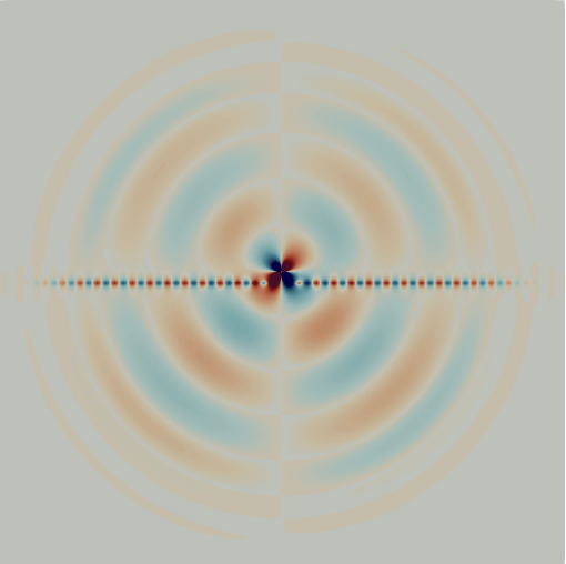
Solution with an interface, absorbing boundary conditions and PML strength 4.
|
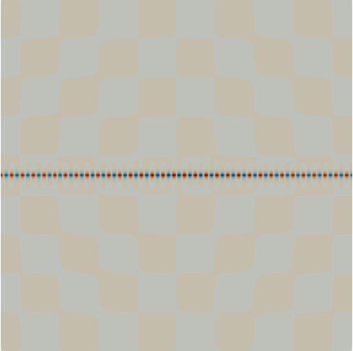
Solution with an interface, Dirichlet boundary conditions and PML strength 0.
| | 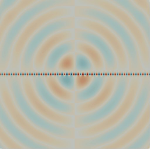
Solution with an interface, absorbing boundary conditions and PML strength 0.
| | 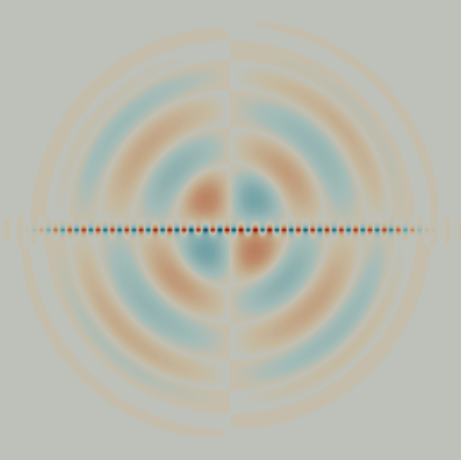
Solution with an interface, absorbing boundary conditions and PML strength 4.
|
The SPP is confined near the interface that we created, however without absorbing boundary conditions, we don't observe a dissipation effect. On adding the absorbing boundary conditions, we observe distortion and resonance and we still don't notice any dissipation. As expected, the PML removes the distortion and resonance. The standing wave is also dissipating and getting absorbed within the PML, and as we increase the PML strength, the standing wave will dissipate more within the PML ring.
Here are some animations to demonstrate the effect of the PML
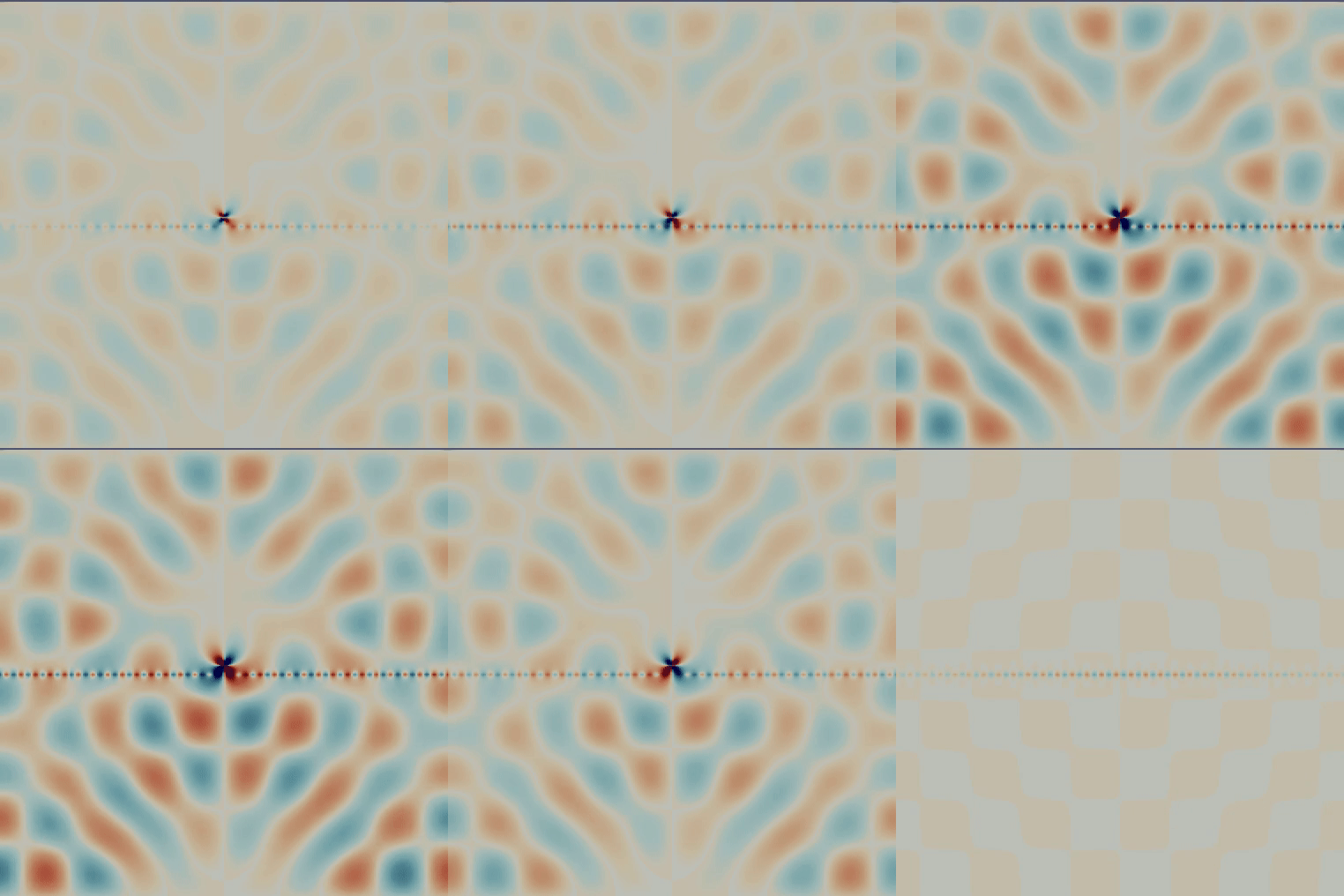
Solution with an interface, Dirichlet boundary conditions and PML strength 0.
| | 
Solution with an interface, absorbing boundary conditions and PML strength 0.
| | 
Solution with an interface, absorbing boundary conditions and PML strength 4.
|
Solution with an interface, Dirichlet boundary conditions and PML strength 0.
| | 
Solution with an interface, absorbing boundary conditions and PML strength 0.
| | 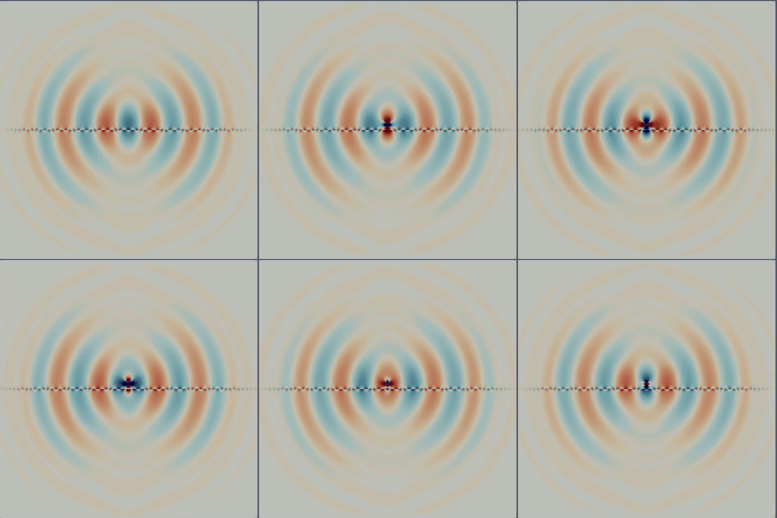
Solution with an interface, absorbing boundary conditions and PML strength 4.
|
Notes
Real and Complex Matrices
As is evident from the results, we are splitting our solution matrices into the real and the imaginary components. We started off using the H^{curl} conforming Nédélec Elements, and we made two copies of the Finite Elements in order to represent the real and the imaginary components of our input (FE_NedelecSZ was used instead of FE_Nedelec to avoid the sign conflicts issues present in traditional Nédélec elements). In the assembly, we create two vectors of dimension dim that assist us in extracting the real and the imaginary components of our finite elements.
Rotations and Scaling
As we see in our assembly, our finite element is rotated and scaled as follows:
const auto phi_i = real_part.value(i, q_point) - 1.0i * imag_part.value(i, q_point);
This \phi_i variable doesn't need to be scaled in this way, we may choose any arbitrary scaling constants a and b. If we choose this scaling, the \phi_j must also be modified with the same scaling, as follows:
const auto phi_i = a*real_part.value(i, q_point) -
bi * imag_part.value(i, q_point);
const auto phi_j = a*real_part.value(i, q_point) +
bi * imag_part.value(i, q_point);
Moreover, the cell_rhs need not be the real part of the rhs_value. Say if we modify to take the imaginary part of the computed rhs_value, we must also modify the cell_matrix accordingly to take the imaginary part of temp. However, making these changes to both sides of the equation will not affect our solution, and we will still be able to generate the surface plasmon polariton.
cell_rhs(i) += rhs_value.imag();
cell_matrix(i) += temp.imag();
Postprocessing
We will create a video demonstrating the wave in motion, which is essentially an implementation of e^{-i\omega t}(Re(E) + i*Im(E)) as we increment time. This is done by slightly changing the output function to generate a series of .vtk files, which will represent out solution wave as we increment time. Introduce an input variable t in the output_results() class as output_results(unsigned int t). Then change the class itself to the following:
template <int dim>
void Maxwell<dim>::output_results(unsigned int t)
{
std::cout << "Running step:" << t << std::endl;
postprocessed.
reinit(solution);
for (unsigned int i = 0; i < dof_handler.n_dofs(); ++i)
{
if (i % 4 == 0)
{
postprocessed[i] =
std::cos(2 * M_PI * 0.04 * t) * solution[i] -
std::sin(2 * M_PI * 0.04 * t) * solution[i + 1];
}
else if (i % 4 == 2)
{
postprocessed[i] =
std::cos(2 * M_PI * 0.04 * t) * solution[i] -
std::sin(2 * M_PI * 0.04 * t) * solution[i + 1];
}
}
const std::string filename =
std::ofstream output(filename);
std::cout << "Done running step:" << t << std::endl;
}
void write_vtk(std::ostream &out) const
void add_data_vector(const VectorType &data, const std::vector< std::string > &names, const DataVectorType type=type_automatic, const std::vector< DataComponentInterpretation::DataComponentInterpretation > &data_component_interpretation={})
virtual void build_patches(const unsigned int n_subdivisions=0)
virtual void reinit(const size_type N, const bool omit_zeroing_entries=false)
std::string int_to_string(const unsigned int value, const unsigned int digits=numbers::invalid_unsigned_int)
::VectorizedArray< Number, width > sin(const ::VectorizedArray< Number, width > &)
Finally, in the run() function, replace output_results() with
for (int t = 0; t <= 100; t++)
{
output_results(t);
}
This would generate 100 solution .vtk files, which can be opened in a group on Paraview and then can be saved as an animation. We used FFMPEG to generate gifs.
Possibilities for Extension
The example step could be extended in a number of different directions.
-
The current program uses a direct solver to solve the linear system. This is efficient for two spatial dimensions where scattering problems up to a few millions degrees of freedom can be solved. In 3D, however, the increased stencil size of the Nedelec element pose a severe limiting factor on the problem size that can be computed. As an alternative, the idea to use iterative solvers can be entertained. This, however requires specialized preconditioners. For example, just using an iterative Krylov space solver (such as SolverGMRES) on above problem will requires many thousands of iterations to converge. Unfortunately, time-harmonic Maxwell's equations lack the usual notion of local smoothing properties, which renders the usual suspects, such as a geometric multigrid (see the Multigrid class), largely useless. A possible extension would be to implement an additive Schwarz preconditioner (based on domain decomposition, see for example [101]), or a sweeping preconditioner (see for example [203]).
-
Another possible extension of the current program is to introduce local mesh refinement (either based on a residual estimator, or based on the dual weighted residual method, see step-14). This is in particular of interest to counter the increased computational cost caused by the scale separation between the SPP and the dipole.
The plain program
#include <fstream>
#include <iostream>
#include <memory>
namespace Step81
{
using namespace std::complex_literals;
template <int dim>
{
public:
Parameters();
using rank0_type = std::complex<double>;
public:
private:
rank2_type epsilon_1;
rank2_type epsilon_2;
std::complex<double> mu_inv_1;
std::complex<double> mu_inv_2;
rank2_type sigma_tensor;
double dipole_radius;
rank0_type dipole_strength;
};
template <int dim>
Parameters<dim>::Parameters()
{
epsilon_1[0][0] = 1.;
epsilon_1[1][1] = 1.;
add_parameter("material 1 epsilon",
epsilon_1,
"relative permittivity of material 1");
epsilon_2[0][0] = 1.;
epsilon_2[1][1] = 1.;
add_parameter("material 2 epsilon",
epsilon_2,
"relative permittivity of material 2");
mu_inv_1 = 1.;
add_parameter("material 1 mu_inv",
mu_inv_1,
"inverse of relative permeability of material 1");
mu_inv_2 = 1.;
add_parameter("material 2 mu_inv",
mu_inv_2,
"inverse of relative permeability of material 2");
sigma_tensor[0][0] = std::complex<double>(0.001, 0.2);
sigma_tensor[1][1] = std::complex<double>(0.001, 0.2);
add_parameter("sigma",
sigma_tensor,
"surface conductivity between material 1 and material 2");
dipole_radius = 0.3;
add_parameter("dipole radius", dipole_radius, "radius of the dipole");
add_parameter("dipole position", dipole_position, "position of the dipole");
add_parameter("dipole orientation",
dipole_orientation,
"orientation of the dipole");
dipole_strength = 1.;
add_parameter("dipole strength", dipole_strength, "strength of the dipole");
}
template <int dim>
typename Parameters<dim>::rank2_type
{
return (material == 1 ? epsilon_1 : epsilon_2);
}
template <int dim>
std::complex<double> Parameters<dim>::mu_inv(
const Point<dim> & ,
{
return (material == 1 ? mu_inv_1 : mu_inv_2);
}
template <int dim>
typename Parameters<dim>::rank2_type
{
return (left == right ? rank2_type() : sigma_tensor);
}
template <int dim>
typename Parameters<dim>::rank1_type
{
rank1_type J_a;
const auto distance = (dipole_position -
point).
norm() / dipole_radius;
if (distance > 1.)
return J_a;
std::cos(distance * M_PI / 2.) / (M_PI / 2. - 2. / M_PI) /
dipole_radius / dipole_radius;
J_a = dipole_strength * dipole_orientation *
scale;
return J_a;
}
template <int dim>
{
public:
static_assert(dim == 2,
"The perfectly matched layer is only implemented in 2d.");
Parameters<dim> parameters;
PerfectlyMatchedLayer();
std::complex<double> d_bar(
const Point<dim> point);
rank2_type rotation(std::complex<double> d_1,
std::complex<double> d_2,
private:
double inner_radius;
double outer_radius;
double strength;
};
template <int dim>
PerfectlyMatchedLayer<dim>::PerfectlyMatchedLayer()
{
inner_radius = 12.;
add_parameter("inner radius",
inner_radius,
"inner radius of the PML shell");
outer_radius = 20.;
add_parameter("outer radius",
outer_radius,
"outer radius of the PML shell");
strength = 8.;
add_parameter("strength", strength, "strength of the PML");
}
template <int dim>
typename std::complex<double>
PerfectlyMatchedLayer<dim>::d(
const Point<dim> point)
{
if (radius > inner_radius)
{
const double s =
strength * ((radius - inner_radius) * (radius - inner_radius)) /
((outer_radius - inner_radius) * (outer_radius - inner_radius));
return {1.0, s};
}
else
{
return 1.0;
}
}
template <int dim>
typename std::complex<double>
PerfectlyMatchedLayer<dim>::d_bar(
const Point<dim> point)
{
if (radius > inner_radius)
{
const double s_bar =
strength / 3. *
((radius - inner_radius) * (radius - inner_radius) *
(radius - inner_radius)) /
(radius * (outer_radius - inner_radius) *
(outer_radius - inner_radius));
return {1.0, s_bar};
}
else
{
return 1.0;
}
}
template <int dim>
typename PerfectlyMatchedLayer<dim>::rank2_type
PerfectlyMatchedLayer<dim>::rotation(std::complex<double> d_1,
std::complex<double> d_2,
{
rank2_type result;
return result;
}
template <int dim>
typename PerfectlyMatchedLayer<dim>::rank2_type
PerfectlyMatchedLayer<dim>::a_matrix(
const Point<dim> point)
{
const auto d = this->
d(point);
const auto d_bar = this->d_bar(point);
return invert(rotation(d * d, d * d_bar, point)) *
rotation(d * d, d * d_bar, point);
}
template <int dim>
typename PerfectlyMatchedLayer<dim>::rank2_type
PerfectlyMatchedLayer<dim>::b_matrix(
const Point<dim> point)
{
const auto d = this->
d(point);
const auto d_bar = this->d_bar(point);
return invert(rotation(d, d_bar, point)) * rotation(d, d_bar, point);
}
template <int dim>
typename PerfectlyMatchedLayer<dim>::rank2_type
PerfectlyMatchedLayer<dim>::c_matrix(
const Point<dim> point)
{
const auto d = this->
d(point);
const auto d_bar = this->d_bar(point);
return invert(rotation(1. / d_bar, 1. / d, point)) *
rotation(1. / d_bar, 1. / d, point);
}
template <int dim>
{
public:
Maxwell();
private:
double scaling;
unsigned int refinements;
unsigned int fe_order;
unsigned int quadrature_order;
bool absorbing_boundary;
void parse_parameters_callback();
void make_grid();
void setup_system();
void assemble_system();
void solve();
void output_results();
Parameters<dim> parameters;
PerfectlyMatchedLayer<dim> perfectly_matched_layer;
std::unique_ptr<FiniteElement<dim>> fe;
};
template <int dim>
Maxwell<dim>::Maxwell()
{
[&]() { parse_parameters_callback(); });
scaling = 20;
add_parameter("scaling", scaling, "scale of the hypercube geometry");
refinements = 8;
add_parameter("refinements",
refinements,
"number of refinements of the geometry");
fe_order = 0;
add_parameter("fe order", fe_order, "order of the finite element space");
quadrature_order = 1;
add_parameter("quadrature order",
quadrature_order,
"order of the quadrature");
absorbing_boundary = true;
add_parameter("absorbing boundary condition",
absorbing_boundary,
"use absorbing boundary conditions?");
}
template <int dim>
void Maxwell<dim>::parse_parameters_callback()
{
}
template <int dim>
void Maxwell<dim>::make_grid()
{
if (!absorbing_boundary)
{
if (face->at_boundary())
face->set_boundary_id(1);
};
cell->set_material_id(1);
else
cell->set_material_id(2);
<< std::endl;
}
template <int dim>
void Maxwell<dim>::setup_system()
{
dof_handler.distribute_dofs(*fe);
std::cout << "Number of degrees of freedom: " << dof_handler.n_dofs()
<< std::endl;
solution.reinit(dof_handler.n_dofs());
system_rhs.reinit(dof_handler.n_dofs());
constraints.clear();
dof_handler,
0,
0,
constraints);
dof_handler,
dim,
0,
constraints);
constraints.close();
dsp,
constraints,
true);
sparsity_pattern.copy_from(dsp);
system_matrix.reinit(sparsity_pattern);
}
template <int dim>
tangential_part(
const Tensor<1, dim, std::complex<double>> &tensor,
{
auto result = tensor;
result[0] = normal[1] * (tensor[0] * normal[1] - tensor[1] * normal[0]);
result[1] = -normal[0] * (tensor[0] * normal[1] - tensor[1] * normal[0]);
return result;
}
template <int dim>
void Maxwell<dim>::assemble_system()
{
const QGauss<dim> quadrature_formula(quadrature_order);
const QGauss<dim - 1> face_quadrature_formula(quadrature_order);
quadrature_formula,
face_quadrature_formula,
const unsigned int dofs_per_cell = fe->dofs_per_cell;
const unsigned int n_q_points = quadrature_formula.size();
const unsigned int n_face_q_points = face_quadrature_formula.size();
std::vector<types::global_dof_index> local_dof_indices(dofs_per_cell);
for (const auto &cell : dof_handler.active_cell_iterators())
{
fe_values.reinit(cell);
cell_rhs = 0.;
cell->get_dof_indices(local_dof_indices);
const auto id = cell->material_id();
for (unsigned int q_point = 0; q_point < n_q_points; ++q_point)
{
auto mu_inv = parameters.mu_inv(position, id);
auto epsilon = parameters.epsilon(position,
id);
const auto J_a = parameters.J_a(position, id);
const auto A = perfectly_matched_layer.a_matrix(position);
const auto B = perfectly_matched_layer.b_matrix(position);
const auto d = perfectly_matched_layer.d(position);
for (const auto i : fe_values.dof_indices())
{
constexpr std::complex<double> imag{0., 1.};
const auto phi_i =
imag * fe_values[imag_part].value(i, q_point);
const auto curl_phi_i =
imag * fe_values[imag_part].curl(i, q_point);
const auto rhs_value =
(imag * scalar_product(J_a, phi_i)) * fe_values.JxW(q_point);
cell_rhs(i) += rhs_value.real();
for (const auto j : fe_values.dof_indices())
{
const auto phi_j =
imag * fe_values[imag_part].value(j, q_point);
const auto curl_phi_j =
imag * fe_values[imag_part].curl(j, q_point);
const auto temp =
(scalar_product(mu_inv * curl_phi_j, curl_phi_i) -
scalar_product(epsilon * phi_j, phi_i)) *
fe_values.JxW(q_point);
}
}
}
for (const auto &face : cell->face_iterators())
{
if (face->at_boundary())
{
const auto id = face->boundary_id();
if (id != 0)
{
fe_face_values.reinit(cell, face);
for (unsigned int q_point = 0; q_point < n_face_q_points;
++q_point)
{
auto mu_inv = parameters.mu_inv(position, id);
auto epsilon = parameters.epsilon(position,
id);
const auto A =
perfectly_matched_layer.a_matrix(position);
const auto B =
perfectly_matched_layer.b_matrix(position);
const auto d = perfectly_matched_layer.d(position);
const auto normal =
fe_face_values.normal_vector(q_point);
for (const auto i : fe_face_values.dof_indices())
{
constexpr std::complex<double> imag{0., 1.};
const auto phi_i =
fe_face_values[
real_part].value(i, q_point) -
imag *
fe_face_values[imag_part].value(i, q_point);
const auto phi_i_T = tangential_part(phi_i, normal);
for (const auto j : fe_face_values.dof_indices())
{
const auto phi_j =
fe_face_values[
real_part].value(j, q_point) +
imag *
fe_face_values[imag_part].value(j, q_point);
const auto phi_j_T =
tangential_part(phi_j, normal) *
fe_face_values.JxW(q_point);
const auto prod = mu_inv *
epsilon;
const auto sqrt_prod = prod;
const auto temp =
-imag * scalar_product((sqrt_prod * phi_j_T),
phi_i_T);
}
}
}
}
}
else
{
const auto face_index = cell->face_iterator_to_index(face);
const auto id1 = cell->material_id();
const auto id2 = cell->neighbor(face_index)->material_id();
if (id1 == id2)
continue;
fe_face_values.reinit(cell, face);
for (unsigned int q_point = 0; q_point < n_face_q_points;
++q_point)
{
auto sigma = parameters.sigma(position, id1, id2);
const auto B = perfectly_matched_layer.b_matrix(position);
const auto C = perfectly_matched_layer.c_matrix(position);
const auto normal = fe_face_values.normal_vector(q_point);
for (const auto i : fe_face_values.dof_indices())
{
constexpr std::complex<double> imag{0., 1.};
const auto phi_i =
fe_face_values[
real_part].value(i, q_point) -
imag * fe_face_values[imag_part].value(i, q_point);
const auto phi_i_T = tangential_part(phi_i, normal);
for (const auto j : fe_face_values.dof_indices())
{
const auto phi_j =
fe_face_values[
real_part].value(j, q_point) +
imag *
fe_face_values[imag_part].value(j, q_point);
const auto phi_j_T = tangential_part(phi_j, normal);
const auto temp =
-imag *
scalar_product((sigma * phi_j_T), phi_i_T) *
fe_face_values.JxW(q_point);
}
}
}
}
}
constraints.distribute_local_to_global(
cell_matrix, cell_rhs, local_dof_indices, system_matrix, system_rhs);
}
}
template <int dim>
void Maxwell<dim>::solve()
{
A_direct.
vmult(solution, system_rhs);
}
template <int dim>
void Maxwell<dim>::output_results()
{
{"real_Ex", "real_Ey", "imag_Ex", "imag_Ey"});
std::ofstream output("solution.vtk");
}
template <int dim>
void Maxwell<dim>::run()
{
make_grid();
setup_system();
assemble_system();
solve();
output_results();
}
}
int main()
{
try
{
Step81::Maxwell<2> maxwell_2d;
maxwell_2d.run();
}
catch (std::exception &exc)
{
std::cerr << std::endl
<< std::endl
<< "----------------------------------------------------"
<< std::endl;
std::cerr << "Exception on processing: " << std::endl
<< exc.what() << std::endl
<< "Aborting!" << std::endl
<< "----------------------------------------------------"
<< std::endl;
return 1;
}
catch (...)
{
std::cerr << std::endl
<< std::endl
<< "----------------------------------------------------"
<< std::endl;
std::cerr << "Unknown exception!" << std::endl
<< "Aborting!" << std::endl
<< "----------------------------------------------------"
<< std::endl;
return 1;
}
return 0;
}
void vmult(Vector< double > &dst, const Vector< double > &src) const
void cell_matrix(FullMatrix< double > &M, const FEValuesBase< dim > &fe, const FEValuesBase< dim > &fetest, const ArrayView< const std::vector< double > > &velocity, const double factor=1.)
void quadrature_points(const Triangulation< dim, spacedim > &triangulation, const Quadrature< dim > &quadrature, const std::vector< std::vector< BoundingBox< spacedim > > > &global_bounding_boxes, ParticleHandler< dim, spacedim > &particle_handler, const Mapping< dim, spacedim > &mapping=(ReferenceCells::get_hypercube< dim >() .template get_default_linear_mapping< dim, spacedim >()), const std::vector< std::vector< double > > &properties={})
SymmetricTensor< 2, dim, Number > C(const Tensor< 2, dim, Number > &F)
SymmetricTensor< 2, dim, Number > epsilon(const Tensor< 2, dim, Number > &Grad_u)
void run(const Iterator &begin, const std_cxx20::type_identity_t< Iterator > &end, Worker worker, Copier copier, const ScratchData &sample_scratch_data, const CopyData &sample_copy_data, const unsigned int queue_length, const unsigned int chunk_size)


