This tutorial depends on step-12.
Introduction
Overview
This example is devoted to anisotropic refinement, which extends to possibilities of local refinement. In most parts, this is a modification of the step-12 tutorial program, we use the same DG method for a linear transport equation. This program will cover the following topics:
-
Anisotropic refinement: What is the meaning of anisotropic refinement?
-
Implementation: Necessary modifications of code to work with anisotropically refined meshes.
-
Jump indicator: A simple indicator for anisotropic refinement in the context of DG methods.
The discretization itself will not be discussed, and neither will implementation techniques not specific to anisotropic refinement used here. Please refer to step-12 for this.
Please note, at the moment of writing this tutorial program, anisotropic refinement is only fully implemented for discontinuous Galerkin Finite Elements. This may later change (or may already have).
- Note
- While this program is a modification of step-12, it is an adaptation of a version of step-12 written early on in the history of deal.II when the MeshWorker framework wasn't available yet. Consequently, it bears little resemblance to the step-12 as it exists now, apart from the fact that it solves the same equation with the same discretization.
Anisotropic refinement
All the adaptive processes in the preceding tutorial programs were based on isotropic refinement of cells, which cuts all edges in half and forms new cells of these split edges (plus some additional edges, faces and vertices, of course). In deal.II, anisotropic refinement refers to the process of splitting only part of the edges while leaving the others unchanged. Consider a simple square cell, for example:
-------*
| |
| |
| |
-------*
After the usual refinement it will consist of four children and look like this:
---*---*
| | |
| | |
---*---*
The new anisotropic refinement may take two forms: either we can split the edges which are parallel to the horizontal x-axis, resulting in these two child cells:
---*---*
| | |
| | |
---*---*
or we can split the two edges which run along the y-axis, resulting again in two children, which look that way, however:
-------*
| |
| |
-------*
All refinement cases of cells are described by an enumeration RefinementPossibilities::Possibilities, and the above anisotropic cases are called cut_x and cut_y for obvious reasons. The isotropic refinement case is called cut_xy in 2D and can be requested from the RefinementCase class via RefinementCase<dim>::isotropic_refinement.
In 3D, there is a third axis which can be split, the z-axis, and thus we have an additional refinement case cut_z here. Isotropic refinement will now refine a cell along the x-, y- and z-axes and thus be referred to as cut_xyz. Additional cases cut_xy, cut_xz and cut_yz exist, which refine a cell along two of the axes, but not along the third one. Given a hex cell with x-axis running to the right, y-axis 'into the page' and z-axis to the top,
-----------*
/ /|
/ / |
/ / |
-----------* |
| | |
| | *
| | /
| | /
| |/
-----------*
we have the isotropic refinement case,
-----*-----*
/ / /|
-----*-----* |
/ / /| *
-----*-----* |/|
| | | * |
| | |/| *
-----*-----* |/
| | | *
| | |/
-----*-----*
three anisotropic cases which refine only one axis:
-----*-----* *-----------* *-----------*
/ / /| / /| / /|
/ / / | *-----------* | / / |
/ / / | / /| | / / *
-----*-----* | *-----------* | | *-----------* /|
| | | | | | | | | | / |
| | | * | | | * | |/ *
| | | / | | |/ *-----------* /
| | | / | | * | | /
| | |/ | |/ | |/
-----*-----* *-----------* *-----------*
and three cases which refine two of the three axes:
-----*-----* *-----*-----* *-----------*
/ / /| / / /| / /|
-----*-----* | / / / | *-----------* |
/ / /| | / / / * / /| *
-----*-----* | | *-----*-----* /| *-----------* |/|
| | | | | | | | / | | | * |
| | | | * | | |/ * | |/| *
| | | |/ *-----*-----* / *-----------* |/
| | | * | | | / | | *
| | |/ | | |/ | |/
-----*-----* *-----*-----* *-----------*
For 1D problems, anisotropic refinement can make no difference, as there is only one coordinate direction for a cell, so it is not possible to split it in any other way than isotropically.
Motivation
Adaptive local refinement is used to obtain fine meshes which are well adapted to solving the problem at hand efficiently. In short, the size of cells which produce a large error is reduced to obtain a better approximation of the solution to the problem at hand. However, a lot of problems contain anisotropic features. Prominent examples are shocks or boundary layers in compressible viscous flows. An efficient mesh approximates these features with cells of higher aspect ratio which are oriented according to the mentioned features. Using only isotropic refinement, the aspect ratios of the original mesh cells are preserved, as they are inherited by the children of a cell. Thus, starting from an isotropic mesh, a boundary layer will be refined in order to catch the rapid variation of the flow field in the wall normal direction, thus leading to cells with very small edge lengths both in normal and tangential direction. Usually, much higher edge lengths in tangential direction and thus significantly less cells could be used without a significant loss in approximation accuracy. An anisotropic refinement process can modify the aspect ratio from mother to child cells by a factor of two for each refinement step. In the course of several refinements, the aspect ratio of the fine cells can be optimized, saving a considerable number of cells and correspondingly degrees of freedom and thus computational resources, memory as well as CPU time.
Implementation
Most of the time, when we do finite element computations, we only consider one cell at a time, for example to calculate cell contributions to the global matrix, or to interpolate boundary values. However, sometimes we have to look at how cells are related in our algorithms. Relationships between cells come in two forms: neighborship and mother-child relationship. For the case of isotropic refinement, deal.II uses certain conventions (invariants) for cell relationships that are always maintained. For example, a refined cell always has exactly 2^{dim} children. And (except for the 1d case), two neighboring cells may differ by at most one refinement level: they are equally often refined or one of them is exactly once more refined, leaving exactly one hanging node on the common face. Almost all of the time these invariants are only of concern in the internal implementation of the library. However, there are cases where knowledge of them is also relevant to an application program.
In the current context, it is worth noting that the kind of mesh refinement affects some of the most fundamental assumptions. Consequently, some of the usual code found in application programs will need modifications to exploit the features of meshes which were created using anisotropic refinement. For those interested in how deal.II evolved, it may be of interest that the loosening of such invariants required some incompatible changes. For example, the library used to have a member GeometryInfo<dim>::children_per_cell that specified how many children a cell has once it is refined. For isotropic refinement, this number is equal to 2^{dim}, as mentioned above. However, for anisotropic refinement, this number does not exist, as is can be either two or four in 2D and two, four or eight in 3D, and the member GeometryInfo<dim>::children_per_cell has consequently been removed. It has now been replaced by GeometryInfo<dim>::max_children_per_cell which specifies the maximum number of children a cell can have. How many children a refined cell has was previously available as static information, but now it depends on the actual refinement state of a cell and can be retrieved using TriaAccessor::n_children(), a call that works equally well for both isotropic and anisotropic refinement. A very similar situation can be found for faces and their subfaces: the pertinent information can be queried using GeometryInfo<dim>::max_children_per_face or face->n_children(), depending on the context.
Another important aspect, and the most important one in this tutorial, is the treatment of neighbor-relations when assembling jump terms on the faces between cells. Looking at the documentation of the assemble_system functions in step-12 we notice, that we need to decide if a neighboring cell is coarser, finer or on the same (refinement) level as our current cell. These decisions do not work in the same way for anisotropic refinement as the information given by the level of a cell is not enough to completely characterize anisotropic cells; for example, are the terminal children of a two-dimensional cell that is first cut in x-direction and whose children are then cut in y-direction on level 2, or are they on level 1 as they would be if the cell would have been refined once isotropically, resulting in the same set of finest cells?
After anisotropic refinement, a coarser neighbor is not necessarily exactly one level below ours, but can pretty much have any level relative to the current one; in fact, it can even be on a higher level even though it is coarser. Thus the decisions have to be made on a different basis, whereas the intention of the decisions stays the same.
In the following, we will discuss the cases that can happen when we want to compute contributions to the matrix (or right hand side) of the form
\int_{\partial K} \varphi_i(x) \varphi_j(x) \; dx
or similar; remember that we integrate terms like this using the FEFaceValues and FESubfaceValues classes. We will also show how to write code that works for both isotropic and anisotropic refinement:
-
Finer neighbor: If we are on an active cell and want to integrate over a face f\subset \partial K, the first possibility is that the neighbor behind this face is more refined, i.e. has children occupying only part of the common face. In this case, the face under consideration has to be a refined one, which can determine by asking if (face->has_children()). If this is true, we need to loop over all subfaces and get the neighbors' child behind this subface, so that we can reinit an FEFaceValues object with the neighbor and an FESubfaceValues object with our cell and the respective subface.
For isotropic refinement, this kind is reasonably simple because we know that an invariant of the isotropically refined adaptive meshes in deal.II is that neighbors can only differ by exactly one refinement level. However, this isn't quite true any more for anisotropically refined meshes, in particular in 3d; there, the active cell we are interested on the other side of f might not actually be a child of our neighbor, but perhaps a grandchild or even a farther offspring. Fortunately, this complexity is hidden in the internals of the library. All we need to do is call the CellAccessor::neighbor_child_on_subface() function. Still, in 3D there are two cases which need special consideration:
-
If the neighbor is refined more than once anisotropically, it might be that here are not two or four but actually three subfaces to consider. Imagine the following refinement process of the (two-dimensional) face of the (three-dimensional) neighbor cell we are considering: first the face is refined along x, later on only the left subface is refined along y.
-------* *---*---* *---*---*
| | | | | | | |
| | ---> | | | ---> *---* |
| | | | | | | |
-------* *---*---* *---*---*
Here the number of subfaces is three. It is important to note the subtle differences between, for a face, TriaAccessor::n_children() and TriaAccessor::n_active_descendants(). The first function returns the number of immediate children, which would be two for the above example, whereas the second returns the number of active offspring (i.e., including children, grandchildren, and further descendants), which is the correct three in the example above. Using face->n_active_descendants() works for isotropic and anisotropic as well as 2D and 3D cases, so it should always be used. It should be noted that if any of the cells behind the two small subfaces on the left side of the rightmost image is further refined, then the current cell (i.e. the side from which we are viewing this common face) is going to be refined as well: this is so because otherwise the invariant of having only one hanging node per edge would be violated.
-
It might be, that the neighbor is coarser, but still has children which are finer than our current cell. This situation can occur if two equally coarse cells are refined, where one of the cells has two children at the face under consideration and the other one four. The cells in the next graphic are only separated from each other to show the individual refinement cases.
-----------* *-----------*
/ /| / /|
############# | +++++++++++++ |
# ## | + ++ *
############# # | +++++++++++++ +/|
# # # | + + + |
# # # * + +++ *
# # #/ +++++++++++++ +/
# # # + + +
# ## + ++
############# +++++++++++++
Here, the left two cells resulted from an anisotropic bisection of the mother cell in y-direction, whereas the right four cells resulted from a simultaneous anisotropic refinement in both the y- and z-directions. The left cell marked with # has two finer neighbors marked with +, but the actual neighbor of the left cell is the complete right mother cell, as the two cells marked with + are finer and their direct mother is the one large cell.
However, fortunately, CellAccessor::neighbor_child_on_subface() takes care of these situations by itself, if you loop over the correct number of subfaces, in the above example this is two. The FESubfaceValues<dim>::reinit function takes care of this too, so that the resulting state is always correct. There is one little caveat, however: For reiniting the neighbors FEFaceValues object you need to know the index of the face that points toward the current cell. Usually you assume that the neighbor you get directly is as coarse or as fine as you, if it has children, thus this information can be obtained with CellAccessor::neighbor_of_neighbor(). If the neighbor is coarser, however, you would have to use the first value in CellAccessor::neighbor_of_coarser_neighbor() instead. In order to make this easy for you, there is CellAccessor::neighbor_face_no() which does the correct thing for you and returns the desired result.
-
Neighbor is as fine as our cell: After we ruled out all cases in which there are finer children, we only need to decide, whether the neighbor is coarser here. For this, there is the CellAccessor::neighbor_is_coarser() function which returns a boolean. In order to get the relevant case of a neighbor of the same coarseness we would use else if (!cell->neighbor_is_coarser(face_no)). The code inside this block can be left untouched. However, there is one thing to mention here: If we want to use a rule, which cell should assemble certain terms on a given face we might think of the rule presented in step-12. We know that we have to leave out the part about comparing our cell's level with that of the neighbor and replace it with the test for a coarser neighbor presented above. However, we also have to consider the possibility that neighboring cells of same coarseness have the same index (on different levels). Thus we have to include the case where the cells have the same index, and give an additional condition, which of the cells should assemble the terms, e.g. we can choose the cell with lower level. The details of this concept can be seen in the implementation below.
-
Coarser neighbor: The remaining case is obvious: If there are no refined neighbors and the neighbor is not as fine as the current cell, then it must be coarser. Thus we can leave the old condition phrase, simply using else. The CellAccessor::neighbor_of_coarser_neighbor() function takes care of all the complexity of anisotropic refinement combined with possible non standard face orientation, flip and rotation on general 3D meshes.
Mesh smoothing
When a triangulation is refined, cells which were not flagged for refinement may be refined nonetheless. This is due to additional smoothing algorithms which are either necessary or requested explicitly. In particular, the restriction that there be at most one hanging node on each edge frequently forces the refinement of additional cells neighboring ones that are already finer and are flagged for further refinement.
However, deal.II also implements a number of algorithms that make sure that resulting meshes are smoother than just the bare minimum, for example ensuring that there are no isolated refined cells surrounded by non-refined ones, since the additional degrees of freedom on these islands would almost all be constrained by hanging node constraints. (See the documentation of the Triangulation class and its Triangulation::MeshSmoothing member for more information on mesh smoothing.)
Most of the smoothing algorithms that were originally developed for the isotropic case have been adapted to work in a very similar way for both anisotropic and isotropic refinement. There are two algorithms worth mentioning, however:
-
MeshSmoothing::limit_level_difference_at_vertices: In an isotropic environment, this algorithm tries to ensure a good approximation quality by reducing the difference in refinement level of cells meeting at a common vertex. However, there is no clear corresponding concept for anisotropic refinement, thus this algorithm may not be used in combination with anisotropic refinement. This restriction is enforced by an assertion which throws an error as soon as the algorithm is called on a triangulation which has been refined anisotropically.
-
MeshSmoothing::allow_anisotropic_smoothing: If refinement is introduced to limit the number of hanging nodes, the additional cells are often not needed to improve the approximation quality. This is especially true for DG methods. If you set the flag allow_anisotropic_smoothing the smoothing algorithm tries to minimize the number of probably unneeded additional cells by using anisotropic refinement for the smoothing. If you set this smoothing flag you might get anisotropically refined cells, even if you never set a single refinement flag to anisotropic refinement. Be aware that you should only use this flag, if your code respects the possibility of anisotropic meshes. Combined with a suitable anisotropic indicator this flag can help save additional cells and thus effort.
Jump indicator
Using the benefits of anisotropic refinement requires an indicator to catch anisotropic features of the solution and exploit them for the refinement process. Generally the anisotropic refinement process will consist of several steps:
-
Calculate an error indicator.
-
Use the error indicator to flag cells for refinement, e.g. using a fixed number or fraction of cells. Those cells will be flagged for isotropic refinement automatically.
-
Evaluate a distinct anisotropic indicator only on the flagged cells.
-
Use the anisotropic indicator to set a new, anisotropic refinement flag for cells where this is appropriate, leave the flags unchanged otherwise.
-
Call Triangulation<dim>::execute_coarsening_and_refinement to perform the requested refinement, using the requested isotropic and anisotropic flags.
This approach is similar to the one we have used in step-27 for hp-refinement and has the great advantage of flexibility: Any error indicator can be used in the anisotropic process, i.e. if you have quite involved a posteriori goal-oriented error indicators available you can use them as easily as a simple Kelly error estimator. The anisotropic part of the refinement process is not influenced by this choice. Furthermore, simply leaving out the third and forth steps leads to the same isotropic refinement you used to get before any anisotropic changes in deal.II or your application program. As a last advantage, working only on cells flagged for refinement results in a faster evaluation of the anisotropic indicator, which can become noticeable on finer meshes with a lot of cells if the indicator is quite involved.
Here, we use a very simple approach which is only applicable to DG methods. The general idea is quite simple: DG methods allow the discrete solution to jump over the faces of a cell, whereas it is smooth within each cell. Of course, in the limit we expect that the jumps tend to zero as we refine the mesh and approximate the true solution better and better. Thus, a large jump across a given face indicates that the cell should be refined (at least) orthogonally to that face, whereas a small jump does not lead to this conclusion. It is possible, of course, that the exact solution is not smooth and that it also features a jump. In that case, however, a large jump over one face indicates, that this face is more or less parallel to the jump and in the vicinity of it, thus again we would expect a refinement orthogonal to the face under consideration to be effective.
The proposed indicator calculates the average jump K_j, i.e. the mean value of the absolute jump |[u]| of the discrete solution u over the two faces f_i^j, i=1,2, j=1..d orthogonal to coordinate direction j on the unit cell.
K_j = \frac{\sum_{i=1}^2 \int_{f_i^j}|[u]| dx}{\sum_{i=1}^2 |f_i^j|} .
If the average jump in one direction is larger than the average of the jumps in the other directions by a certain factor \kappa, i.e. if K_i > \kappa \frac 1{d-1} \sum_{j=1, j\neq i}^d K_j, the cell is refined only along that particular direction i, otherwise the cell is refined isotropically.
Such a criterion is easily generalized to systems of equations: the absolute value of the jump would be replaced by an appropriate norm of the vector-valued jump.
The problem
We solve the linear transport equation presented in step-12. The domain is extended to cover [-1,1]\times[0,1] in 2D, where the flow field \beta describes a counterclockwise quarter circle around the origin in the right half of the domain and is parallel to the x-axis in the left part of the domain. The inflow boundary is again located at x=1 and along the positive part of the x-axis, and the boundary conditions are chosen as in step-12.
The commented program
The deal.II include files have already been covered in previous examples and will thus not be further commented on.
#include <deal.II/base/function.h>
#include <deal.II/base/quadrature_lib.h>
#include <deal.II/base/timer.h>
#include <deal.II/lac/precondition_block.h>
#include <deal.II/lac/solver_richardson.h>
#include <deal.II/lac/sparse_matrix.h>
#include <deal.II/lac/vector.h>
#include <deal.II/grid/tria.h>
#include <deal.II/grid/grid_generator.h>
#include <deal.II/grid/grid_out.h>
#include <deal.II/grid/grid_refinement.h>
#include <deal.II/dofs/dof_handler.h>
#include <deal.II/dofs/dof_tools.h>
#include <deal.II/fe/fe_values.h>
#include <deal.II/fe/mapping_q1.h>
#include <deal.II/fe/fe_dgq.h>
#include <deal.II/numerics/data_out.h>
#include <deal.II/numerics/derivative_approximation.h>
And this again is C++:
#include <array>
#include <iostream>
#include <fstream>
The last step is as in all previous programs:
Equation data
The classes describing equation data and the actual assembly of individual terms are almost entirely copied from step-12. We will comment on differences.
template <int dim>
{
public:
std::vector<double> &values,
const unsigned int = 0) const override
{
(void)points;
std::fill(values.begin(), values.end(), 0.);
}
};
template <int dim>
class BoundaryValues :
public Function<dim>
{
public:
std::vector<double> &values,
const unsigned int = 0) const override
{
for (unsigned int i = 0; i < values.size(); ++i)
{
if (points[i][0] < 0.5)
values[i] = 1.;
else
values[i] = 0.;
}
}
};
template <int dim>
class Beta
{
public:
virtual void value_list(const std::vector< Point< dim > > &points, std::vector< RangeNumberType > &values, const unsigned int component=0) const
#define AssertDimension(dim1, dim2)
The flow field is chosen to be a quarter circle with counterclockwise flow direction and with the origin as midpoint for the right half of the domain with positive x values, whereas the flow simply goes to the left in the left part of the domain at a velocity that matches the one coming in from the right. In the circular part the magnitude of the flow velocity is proportional to the distance from the origin. This is a difference to step-12, where the magnitude was 1 everywhere. the new definition leads to a linear variation of \beta along each given face of a cell. On the other hand, the solution u(x,y) is exactly the same as before.
void value_list(
const std::vector<
Point<dim>> &points,
{
for (unsigned int i = 0; i < points.size(); ++i)
{
if (points[i][0] > 0)
{
values[i][0] = -points[i][1];
values[i][1] = points[i][0];
}
else
{
values[i][0] = -points[i][1];
}
}
}
};
Class: DGTransportEquation
This declaration of this class is utterly unaffected by our current changes.
template <int dim>
class DGTransportEquation
{
public:
DGTransportEquation();
private:
const Beta<dim> beta_function;
const RHS<dim> rhs_function;
const BoundaryValues<dim> boundary_function;
};
Likewise, the constructor of the class as well as the functions assembling the terms corresponding to cell interiors and boundary faces are unchanged from before. The function that assembles face terms between cells also did not change because all it does is operate on two objects of type FEFaceValuesBase (which is the base class of both FEFaceValues and FESubfaceValues). Where these objects come from, i.e. how they are initialized, is of no concern to this function: it simply assumes that the quadrature points on faces or subfaces represented by the two objects correspond to the same points in physical space.
template <int dim>
DGTransportEquation<dim>::DGTransportEquation()
: beta_function()
, rhs_function()
, boundary_function()
{}
template <int dim>
void DGTransportEquation<dim>::assemble_cell_term(
{
const std::vector<double> &JxW = fe_v.get_JxW_values();
std::vector<Point<dim>> beta(fe_v.n_quadrature_points);
std::vector<double> rhs(fe_v.n_quadrature_points);
beta_function.value_list(fe_v.get_quadrature_points(), beta);
rhs_function.value_list(fe_v.get_quadrature_points(), rhs);
for (unsigned int point = 0; point < fe_v.n_quadrature_points; ++point)
for (unsigned int i = 0; i < fe_v.dofs_per_cell; ++i)
{
for (unsigned int j = 0; j < fe_v.dofs_per_cell; ++j)
ui_vi_matrix(i, j) -= beta[point] * fe_v.shape_grad(i, point) *
fe_v.shape_value(j, point) * JxW[point];
cell_vector(i) +=
rhs[point] * fe_v.shape_value(i, point) * JxW[point];
}
}
template <int dim>
void DGTransportEquation<dim>::assemble_boundary_term(
{
const std::vector<double> &JxW = fe_v.get_JxW_values();
const std::vector<Tensor<1, dim>> &normals = fe_v.get_normal_vectors();
std::vector<Point<dim>> beta(fe_v.n_quadrature_points);
std::vector<double> g(fe_v.n_quadrature_points);
beta_function.value_list(fe_v.get_quadrature_points(), beta);
boundary_function.value_list(fe_v.get_quadrature_points(), g);
for (
unsigned int point = 0;
point < fe_v.n_quadrature_points; ++
point)
{
const double beta_n = beta[
point] * normals[
point];
if (beta_n > 0)
for (unsigned int i = 0; i < fe_v.dofs_per_cell; ++i)
for (unsigned int j = 0; j < fe_v.dofs_per_cell; ++j)
ui_vi_matrix(i, j) += beta_n * fe_v.shape_value(j, point) *
fe_v.shape_value(i, point) * JxW[
point];
else
for (unsigned int i = 0; i < fe_v.dofs_per_cell; ++i)
cell_vector(i) -=
beta_n * g[
point] * fe_v.shape_value(i, point) * JxW[
point];
}
}
template <int dim>
void DGTransportEquation<dim>::assemble_face_term(
{
const std::vector<double> &JxW = fe_v.get_JxW_values();
const std::vector<Tensor<1, dim>> &normals = fe_v.get_normal_vectors();
std::vector<Point<dim>> beta(fe_v.n_quadrature_points);
beta_function.value_list(fe_v.get_quadrature_points(), beta);
for (
unsigned int point = 0;
point < fe_v.n_quadrature_points; ++
point)
{
const double beta_n = beta[
point] * normals[
point];
if (beta_n > 0)
{
for (unsigned int i = 0; i < fe_v.dofs_per_cell; ++i)
for (unsigned int j = 0; j < fe_v.dofs_per_cell; ++j)
ui_vi_matrix(i, j) += beta_n * fe_v.shape_value(j, point) *
fe_v.shape_value(i, point) * JxW[
point];
for (unsigned int k = 0; k < fe_v_neighbor.dofs_per_cell; ++k)
for (unsigned int j = 0; j < fe_v.dofs_per_cell; ++j)
ui_ve_matrix(k, j) -= beta_n * fe_v.shape_value(j, point) *
fe_v_neighbor.shape_value(k, point) *
}
else
{
for (unsigned int i = 0; i < fe_v.dofs_per_cell; ++i)
for (
unsigned int l = 0;
l < fe_v_neighbor.dofs_per_cell; ++
l)
ue_vi_matrix(i, l) += beta_n *
fe_v_neighbor.shape_value(l, point) *
fe_v.shape_value(i, point) * JxW[
point];
for (unsigned int k = 0; k < fe_v_neighbor.dofs_per_cell; ++k)
for (
unsigned int l = 0;
l < fe_v_neighbor.dofs_per_cell; ++
l)
ue_ve_matrix(k, l) -=
beta_n * fe_v_neighbor.shape_value(l, point) *
fe_v_neighbor.shape_value(k, point) * JxW[
point];
}
}
}
Point< spacedim > point(const gp_Pnt &p, const double tolerance=1e-10)
Tensor< 2, dim, Number > l(const Tensor< 2, dim, Number > &F, const Tensor< 2, dim, Number > &dF_dt)
Class: DGMethod
This declaration is much like that of step-12. However, we introduce a new routine (set_anisotropic_flags) and modify another one (refine_grid).
template <int dim>
class DGMethod
{
public:
DGMethod(const bool anisotropic);
void run();
private:
void setup_system();
void assemble_system();
void refine_grid();
void set_anisotropic_flags();
void output_results(const unsigned int cycle) const;
const ::parallel::distributed::Triangulation< dim, spacedim > * triangulation
Again we want to use DG elements of degree 1 (but this is only specified in the constructor). If you want to use a DG method of a different degree replace 1 in the constructor by the new degree.
const unsigned int degree;
This is new, the threshold value used in the evaluation of the anisotropic jump indicator explained in the introduction. Its value is set to 3.0 in the constructor, but it can easily be changed to a different value greater than 1.
const double anisotropic_threshold_ratio;
This is a bool flag indicating whether anisotropic refinement shall be used or not. It is set by the constructor, which takes an argument of the same name.
const bool anisotropic;
const QGauss<dim - 1> face_quadrature;
const DGTransportEquation<dim> dg;
};
template <int dim>
DGMethod<dim>::DGMethod(const bool anisotropic)
: mapping()
,
Change here for DG methods of different degrees.
degree(1)
, fe(degree)
, anisotropic_threshold_ratio(3.)
, anisotropic(anisotropic)
,
As beta is a linear function, we can choose the degree of the quadrature for which the resulting integration is correct. Thus, we choose to use degree+1 Gauss points, which enables us to integrate exactly polynomials of degree 2*degree+1, enough for all the integrals we will perform in this program.
quadrature(degree + 1)
, face_quadrature(degree + 1)
, dg()
{}
template <int dim>
void DGMethod<dim>::setup_system()
{
dof_handler.distribute_dofs(fe);
sparsity_pattern.reinit(dof_handler.n_dofs(),
dof_handler.n_dofs(),
1) *
fe.n_dofs_per_cell());
sparsity_pattern.compress();
system_matrix.reinit(sparsity_pattern);
solution2.reinit(dof_handler.n_dofs());
right_hand_side.reinit(dof_handler.n_dofs());
}
void make_flux_sparsity_pattern(const DoFHandler< dim, spacedim > &dof_handler, SparsityPatternBase &sparsity_pattern)
Function: assemble_system
We proceed with the assemble_system function that implements the DG discretization. This function does the same thing as the assemble_system function from step-12 (but without MeshWorker). The four cases considered for the neighbor-relations of a cell are the same as the isotropic case, namely a) cell is at the boundary, b) there are finer neighboring cells, c) the neighbor is neither coarser nor finer and d) the neighbor is coarser. However, the way in which we decide upon which case we have are modified in the way described in the introduction.
template <int dim>
void DGMethod<dim>::assemble_system()
{
const unsigned int dofs_per_cell = dof_handler.get_fe().n_dofs_per_cell();
std::vector<types::global_dof_index> dofs(dofs_per_cell);
std::vector<types::global_dof_index> dofs_neighbor(dofs_per_cell);
fe,
face_quadrature,
face_update_flags);
fe,
face_quadrature,
face_update_flags);
fe,
face_quadrature,
neighbor_face_update_flags);
for (const auto &cell : dof_handler.active_cell_iterators())
{
ui_vi_matrix = 0;
cell_vector = 0;
fe_v.reinit(cell);
dg.assemble_cell_term(fe_v, ui_vi_matrix, cell_vector);
cell->get_dof_indices(dofs);
for (const auto face_no : cell->face_indices())
{
const auto face = cell->face(face_no);
@ update_values
Shape function values.
@ update_normal_vectors
Normal vectors.
@ update_JxW_values
Transformed quadrature weights.
@ update_gradients
Shape function gradients.
@ update_quadrature_points
Transformed quadrature points.
Case (a): The face is at the boundary.
if (face->at_boundary())
{
fe_v_face.reinit(cell, face_no);
dg.assemble_boundary_term(fe_v_face, ui_vi_matrix, cell_vector);
}
else
{
ExcInternalError());
const auto neighbor = cell->neighbor(face_no);
#define Assert(cond, exc)
@ valid
Iterator points to a valid object.
Case (b): This is an internal face and the neighbor is refined (which we can test by asking whether the face of the current cell has children). In this case, we will need to integrate over the "sub-faces", i.e., the children of the face of the current cell.
(There is a slightly confusing corner case: If we are in 1d – where admittedly the current program and its demonstration of anisotropic refinement is not particularly relevant – then the faces between cells are always the same: they are just vertices. In other words, in 1d, we do not want to treat faces between cells of different level differently. The condition face->has_children() we check here ensures this: in 1d, this function always returns false, and consequently in 1d we will not ever go into this if branch. But we will have to come back to this corner case below in case (c).)
if (face->has_children())
{
We need to know, which of the neighbors faces points in the direction of our cell. Using the neighbor_face_no function we get this information for both coarser and non-coarser neighbors.
const unsigned int neighbor2 =
cell->neighbor_face_no(face_no);
Now we loop over all subfaces, i.e. the children and possibly grandchildren of the current face.
for (unsigned int subface_no = 0;
subface_no < face->n_active_descendants();
++subface_no)
{
To get the cell behind the current subface we can use the neighbor_child_on_subface function. it takes care of all the complicated situations of anisotropic refinement and non-standard faces.
const auto neighbor_child =
cell->neighbor_child_on_subface(face_no, subface_no);
Assert(!neighbor_child->has_children(),
ExcInternalError());
The remaining part of this case is unchanged.
ue_vi_matrix = 0;
ui_ve_matrix = 0;
ue_ve_matrix = 0;
fe_v_subface.reinit(cell, face_no, subface_no);
fe_v_face_neighbor.reinit(neighbor_child, neighbor2);
dg.assemble_face_term(fe_v_subface,
fe_v_face_neighbor,
ui_vi_matrix,
ue_vi_matrix,
ui_ve_matrix,
ue_ve_matrix);
neighbor_child->get_dof_indices(dofs_neighbor);
for (unsigned int i = 0; i < dofs_per_cell; ++i)
for (unsigned int j = 0; j < dofs_per_cell; ++j)
{
system_matrix.add(dofs[i],
dofs_neighbor[j],
ue_vi_matrix(i, j));
system_matrix.add(dofs_neighbor[i],
dofs[j],
ui_ve_matrix(i, j));
system_matrix.add(dofs_neighbor[i],
dofs_neighbor[j],
ue_ve_matrix(i, j));
}
}
}
else
{
Case (c). We get here if this is an internal face and if the neighbor is not further refined (or, as mentioned above, we are in 1d in which case we get here for every internal face). We then need to decide whether we want to integrate over the current face. If the neighbor is in fact coarser, then we ignore the face and instead handle it when we visit the neighboring cell and look at the current face (except in 1d, where as mentioned above this is not happening):
if (dim > 1 && cell->neighbor_is_coarser(face_no))
continue;
On the other hand, if the neighbor is more refined, then we have already handled the face in case (b) above (except in 1d). So for 2d and 3d, we just have to decide whether we want to handle a face between cells at the same level from the current side or from the neighboring side. We do this by introducing a tie-breaker: We'll just take the cell with the smaller index (within the current refinement level). In 1d, we take either the coarser cell, or if they are on the same level, the one with the smaller index within that level. This leads to a complicated condition that, hopefully, makes sense given the description above:
if (((dim > 1) && (cell->index() < neighbor->index())) ||
((dim == 1) && ((cell->level() < neighbor->level()) ||
((cell->level() == neighbor->level()) &&
(cell->index() < neighbor->index())))))
{
Here we know, that the neighbor is not coarser so we can use the usual neighbor_of_neighbor function. However, we could also use the more general neighbor_face_no function.
const unsigned int neighbor2 =
cell->neighbor_of_neighbor(face_no);
ue_vi_matrix = 0;
ui_ve_matrix = 0;
ue_ve_matrix = 0;
fe_v_face.reinit(cell, face_no);
fe_v_face_neighbor.reinit(neighbor, neighbor2);
dg.assemble_face_term(fe_v_face,
fe_v_face_neighbor,
ui_vi_matrix,
ue_vi_matrix,
ui_ve_matrix,
ue_ve_matrix);
neighbor->get_dof_indices(dofs_neighbor);
for (unsigned int i = 0; i < dofs_per_cell; ++i)
for (unsigned int j = 0; j < dofs_per_cell; ++j)
{
system_matrix.add(dofs[i],
dofs_neighbor[j],
ue_vi_matrix(i, j));
system_matrix.add(dofs_neighbor[i],
dofs[j],
ui_ve_matrix(i, j));
system_matrix.add(dofs_neighbor[i],
dofs_neighbor[j],
ue_ve_matrix(i, j));
}
}
We do not need to consider a case (d), as those faces are treated 'from the other side within case (b).
}
}
}
for (unsigned int i = 0; i < dofs_per_cell; ++i)
for (unsigned int j = 0; j < dofs_per_cell; ++j)
system_matrix.add(dofs[i], dofs[j], ui_vi_matrix(i, j));
for (unsigned int i = 0; i < dofs_per_cell; ++i)
right_hand_side(dofs[i]) += cell_vector(i);
}
}
Solver
For this simple problem we use the simple Richardson iteration again. The solver is completely unaffected by our anisotropic changes.
template <int dim>
{
preconditioner.
initialize(system_matrix, fe.n_dofs_per_cell());
solver.solve(system_matrix, solution, right_hand_side, preconditioner);
}
void initialize(const MatrixType &A, const AdditionalData parameters)
Refinement
We refine the grid according to the same simple refinement criterion used in step-12, namely an approximation to the gradient of the solution.
template <int dim>
void DGMethod<dim>::refine_grid()
{
unsigned int n_active_cells() const
We approximate the gradient,
dof_handler,
solution2,
gradient_indicator);
void approximate_gradient(const Mapping< dim, spacedim > &mapping, const DoFHandler< dim, spacedim > &dof, const InputVector &solution, Vector< float > &derivative_norm, const unsigned int component=0)
and scale it to obtain an error indicator.
gradient_indicator[cell->active_cell_index()] *=
std::pow(cell->diameter(), 1 + 1.0 * dim / 2);
Then we use this indicator to flag the 30 percent of the cells with highest error indicator to be refined.
gradient_indicator,
0.3,
0.1);
void refine_and_coarsen_fixed_number(Triangulation< dim, spacedim > &triangulation, const Vector< Number > &criteria, const double top_fraction_of_cells, const double bottom_fraction_of_cells, const unsigned int max_n_cells=std::numeric_limits< unsigned int >::max())
Now the refinement flags are set for those cells with a large error indicator. If nothing is done to change this, those cells will be refined isotropically. If the anisotropic flag given to this function is set, we now call the set_anisotropic_flags() function, which uses the jump indicator to reset some of the refinement flags to anisotropic refinement.
if (anisotropic)
set_anisotropic_flags();
Now execute the refinement considering anisotropic as well as isotropic refinement flags.
}
virtual void execute_coarsening_and_refinement() override
Once an error indicator has been evaluated and the cells with largest error are flagged for refinement we want to loop over the flagged cells again to decide whether they need isotropic refinement or whether anisotropic refinement is more appropriate. This is the anisotropic jump indicator explained in the introduction.
template <int dim>
void DGMethod<dim>::set_anisotropic_flags()
{
We want to evaluate the jump over faces of the flagged cells, so we need some objects to evaluate values of the solution on faces.
fe,
face_quadrature,
face_update_flags);
fe,
face_quadrature,
face_update_flags);
fe,
face_quadrature,
Now we need to loop over all active cells.
for (const auto &cell : dof_handler.active_cell_iterators())
We only need to consider cells which are flagged for refinement.
if (cell->refine_flag_set())
{
std::array<double, dim> jump_in_coordinate_direction;
std::array<double, dim> face_area_in_coordinate_direction;
for (const auto face_no : cell->face_indices())
{
const auto face = cell->face(face_no);
if (!face->at_boundary())
{
Assert(cell->neighbor(face_no).state() ==
ExcInternalError());
const auto neighbor = cell->neighbor(face_no);
std::vector<double> u(fe_v_face.n_quadrature_points);
std::vector<double> u_neighbor(fe_v_face.n_quadrature_points);
The four cases of different neighbor relations seen in the assembly routines are repeated much in the same way here.
if (face->has_children())
{
The neighbor is refined. First we store the information, which of the neighbor's faces points in the direction of our current cell. This property is inherited to the children.
unsigned int neighbor2 = cell->neighbor_face_no(face_no);
Now we loop over all subfaces,
for (unsigned int subface_no = 0;
subface_no < face->n_active_descendants();
++subface_no)
{
get an iterator pointing to the cell behind the present subface...
const auto neighbor_child =
cell->neighbor_child_on_subface(face_no,
subface_no);
Assert(!neighbor_child->has_children(),
ExcInternalError());
... and reinit the respective FEFaceValues and FESubFaceValues objects.
fe_v_subface.reinit(cell, face_no, subface_no);
fe_v_face_neighbor.reinit(neighbor_child, neighbor2);
We obtain the function values
fe_v_subface.get_function_values(solution2, u);
fe_v_face_neighbor.get_function_values(solution2,
u_neighbor);
as well as the quadrature weights, multiplied by the Jacobian determinant.
const std::vector<double> &JxW =
fe_v_subface.get_JxW_values();
Now we loop over all quadrature points
for (unsigned int x = 0;
x < fe_v_subface.n_quadrature_points;
++x)
{
and integrate the absolute value of the jump of the solution, i.e. the absolute value of the difference between the function value seen from the current cell and the neighboring cell, respectively. We know, that the first two faces are orthogonal to the first coordinate direction on the unit cell, the second two faces are orthogonal to the second coordinate direction and so on, so we accumulate these values into vectors with dim components.
jump_in_coordinate_direction[face_no / 2] +=
std::abs(u[x] - u_neighbor[x]) * JxW[x];
::VectorizedArray< Number, width > abs(const ::VectorizedArray< Number, width > &)
We also sum up the scaled weights to obtain the measure of the face.
face_area_in_coordinate_direction[face_no / 2] +=
JxW[x];
}
}
}
else
{
if (!cell->neighbor_is_coarser(face_no))
{
Our current cell and the neighbor have the same refinement along the face under consideration. Apart from that, we do much the same as with one of the subcells in the above case.
unsigned int neighbor2 =
cell->neighbor_of_neighbor(face_no);
fe_v_face.reinit(cell, face_no);
fe_v_face_neighbor.reinit(neighbor, neighbor2);
fe_v_face.get_function_values(solution2, u);
fe_v_face_neighbor.get_function_values(solution2,
u_neighbor);
const std::vector<double> &JxW =
fe_v_face.get_JxW_values();
for (unsigned int x = 0;
x < fe_v_face.n_quadrature_points;
++x)
{
jump_in_coordinate_direction[face_no / 2] +=
std::abs(u[x] - u_neighbor[x]) * JxW[x];
face_area_in_coordinate_direction[face_no / 2] +=
JxW[x];
}
}
else
{
Now the neighbor is actually coarser. This case is new, in that it did not occur in the assembly routine. Here, we have to consider it, but this is not overly complicated. We simply use the neighbor_of_coarser_neighbor function, which again takes care of anisotropic refinement and non-standard face orientation by itself.
std::pair<unsigned int, unsigned int>
neighbor_face_subface =
cell->neighbor_of_coarser_neighbor(face_no);
Assert(neighbor_face_subface.first < cell->n_faces(),
ExcInternalError());
Assert(neighbor_face_subface.second <
neighbor->face(neighbor_face_subface.first)
->n_active_descendants(),
ExcInternalError());
Assert(neighbor->neighbor_child_on_subface(
neighbor_face_subface.first,
neighbor_face_subface.second) == cell,
ExcInternalError());
fe_v_face.reinit(cell, face_no);
fe_v_subface.reinit(neighbor,
neighbor_face_subface.first,
neighbor_face_subface.second);
fe_v_face.get_function_values(solution2, u);
fe_v_subface.get_function_values(solution2,
u_neighbor);
const std::vector<double> &JxW =
fe_v_face.get_JxW_values();
for (unsigned int x = 0;
x < fe_v_face.n_quadrature_points;
++x)
{
jump_in_coordinate_direction[face_no / 2] +=
std::abs(u[x] - u_neighbor[x]) * JxW[x];
face_area_in_coordinate_direction[face_no / 2] +=
JxW[x];
}
}
}
}
}
Now we analyze the size of the mean jumps, which we get dividing the jumps by the measure of the respective faces.
std::array<double, dim> average_jumps;
double sum_of_average_jumps = 0.;
for (unsigned int i = 0; i < dim; ++i)
{
average_jumps[i] = jump_in_coordinate_direction[i] /
face_area_in_coordinate_direction[i];
sum_of_average_jumps += average_jumps[i];
}
Now we loop over the dim coordinate directions of the unit cell and compare the average jump over the faces orthogonal to that direction with the average jumps over faces orthogonal to the remaining direction(s). If the first is larger than the latter by a given factor, we refine only along hat axis. Otherwise we leave the refinement flag unchanged, resulting in isotropic refinement.
for (unsigned int i = 0; i < dim; ++i)
if (average_jumps[i] > anisotropic_threshold_ratio *
(sum_of_average_jumps - average_jumps[i]))
}
}
The Rest
The remaining part of the program very much follows the scheme of previous tutorial programs. We output the mesh in VTU format (just as we did in step-1, for example), and the visualization output in VTU format as we almost always do.
template <int dim>
void DGMethod<dim>::output_results(const unsigned int cycle) const
{
std::string refine_type;
if (anisotropic)
refine_type = ".aniso";
else
refine_type = ".iso";
{
const std::string filename =
"grid-" + std::to_string(cycle) + refine_type + ".svg";
std::cout << " Writing grid to <" << filename << ">..." << std::endl;
std::ofstream svg_output(filename);
}
{
const std::string filename =
"sol-" + std::to_string(cycle) + refine_type + ".vtu";
std::cout << " Writing solution to <" << filename << ">..."
<< std::endl;
std::ofstream gnuplot_output(filename);
data_out.add_data_vector(solution2, "u");
data_out.build_patches(degree);
data_out.write_vtu(gnuplot_output);
}
}
template <int dim>
void DGMethod<dim>::run()
{
for (unsigned int cycle = 0; cycle < 6; ++cycle)
{
std::cout << "Cycle " << cycle << ':' << std::endl;
if (cycle == 0)
{
void attach_dof_handler(const DoFHandler< dim, spacedim > &)
void write_svg(const Triangulation< 2, 2 > &tria, std::ostream &out) const
Create the rectangular domain.
p1[0] = -1.;
for (unsigned int i = 0; i < dim; ++i)
p2[i] = 1.;
Adjust the number of cells in different directions to obtain completely isotropic cells for the original mesh.
std::vector<unsigned int> repetitions(dim, 1);
repetitions[0] = 2;
repetitions,
p1,
p2);
}
else
refine_grid();
std::cout << " Number of active cells: "
setup_system();
std::cout << " Number of degrees of freedom: " << dof_handler.n_dofs()
<< std::endl;
assemble_system();
std::cout << " Time of assemble_system: " << assemble_timer.cpu_time()
<< std::endl;
solve(solution2);
output_results(cycle);
std::cout << std::endl;
}
}
}
int main()
{
try
{
using namespace Step30;
void refine_global(const unsigned int times=1)
void subdivided_hyper_rectangle(Triangulation< dim, spacedim > &tria, const std::vector< unsigned int > &repetitions, const Point< dim > &p1, const Point< dim > &p2, const bool colorize=false)
If you want to run the program in 3d, simply change the following line to const unsigned int dim = 3;.
const unsigned int dim = 2;
{
First, we perform a run with isotropic refinement.
std::cout << "Performing a " << dim
<< "D run with isotropic refinement..." << std::endl
<< "------------------------------------------------"
<< std::endl;
DGMethod<dim> dgmethod_iso(false);
dgmethod_iso.run();
}
{
Now we do a second run, this time with anisotropic refinement.
std::cout << std::endl
<< "Performing a " << dim
<< "D run with anisotropic refinement..." << std::endl
<< "--------------------------------------------------"
<< std::endl;
DGMethod<dim> dgmethod_aniso(true);
dgmethod_aniso.run();
}
}
catch (std::exception &exc)
{
std::cerr << std::endl
<< std::endl
<< "----------------------------------------------------"
<< std::endl;
std::cerr << "Exception on processing: " << std::endl
<< exc.what() << std::endl
<< "Aborting!" << std::endl
<< "----------------------------------------------------"
<< std::endl;
return 1;
}
catch (...)
{
std::cerr << std::endl
<< std::endl
<< "----------------------------------------------------"
<< std::endl;
std::cerr << "Unknown exception!" << std::endl
<< "Aborting!" << std::endl
<< "----------------------------------------------------"
<< std::endl;
return 1;
};
return 0;
}
Results
The output of this program consist of the console output, the SVG files containing the grids, and the solutions given in VTU format.
Performing a 2D run with isotropic refinement...
------------------------------------------------
Cycle 0:
Number of active cells: 128
Number of degrees of freedom: 512
Time of assemble_system: 0.092049
Writing grid to <grid-0.iso.svg>...
Writing solution to <sol-0.iso.vtu>...
Cycle 1:
Number of active cells: 239
Number of degrees of freedom: 956
Time of assemble_system: 0.109519
Writing grid to <grid-1.iso.svg>...
Writing solution to <sol-1.iso.vtu>...
Cycle 2:
Number of active cells: 491
Number of degrees of freedom: 1964
Time of assemble_system: 0.08303
Writing grid to <grid-2.iso.svg>...
Writing solution to <sol-2.iso.vtu>...
Cycle 3:
Number of active cells: 1031
Number of degrees of freedom: 4124
Time of assemble_system: 0.278987
Writing grid to <grid-3.iso.svg>...
Writing solution to <sol-3.iso.vtu>...
Cycle 4:
Number of active cells: 2027
Number of degrees of freedom: 8108
Time of assemble_system: 0.305869
Writing grid to <grid-4.iso.svg>...
Writing solution to <sol-4.iso.vtu>...
Cycle 5:
Number of active cells: 4019
Number of degrees of freedom: 16076
Time of assemble_system: 0.47616
Writing grid to <grid-5.iso.svg>...
Writing solution to <sol-5.iso.vtu>...
Performing a 2D run with anisotropic refinement...
--------------------------------------------------
Cycle 0:
Number of active cells: 128
Number of degrees of freedom: 512
Time of assemble_system: 0.052866
Writing grid to <grid-0.aniso.svg>...
Writing solution to <sol-0.aniso.vtu>...
Cycle 1:
Number of active cells: 171
Number of degrees of freedom: 684
Time of assemble_system: 0.050917
Writing grid to <grid-1.aniso.svg>...
Writing solution to <sol-1.aniso.vtu>...
Cycle 2:
Number of active cells: 255
Number of degrees of freedom: 1020
Time of assemble_system: 0.064132
Writing grid to <grid-2.aniso.svg>...
Writing solution to <sol-2.aniso.vtu>...
Cycle 3:
Number of active cells: 394
Number of degrees of freedom: 1576
Time of assemble_system: 0.119849
Writing grid to <grid-3.aniso.svg>...
Writing solution to <sol-3.aniso.vtu>...
Cycle 4:
Number of active cells: 648
Number of degrees of freedom: 2592
Time of assemble_system: 0.218244
Writing grid to <grid-4.aniso.svg>...
Writing solution to <sol-4.aniso.vtu>...
Cycle 5:
Number of active cells: 1030
Number of degrees of freedom: 4120
Time of assemble_system: 0.128121
Writing grid to <grid-5.aniso.svg>...
Writing solution to <sol-5.aniso.vtu>...
This text output shows the reduction in the number of cells which results from the successive application of anisotropic refinement. After the last refinement step the savings have accumulated so much that almost four times as many cells and thus degrees of freedom are needed in the isotropic case. The time needed for assembly scales with a similar factor.
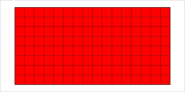
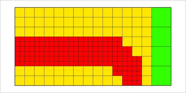
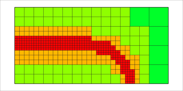
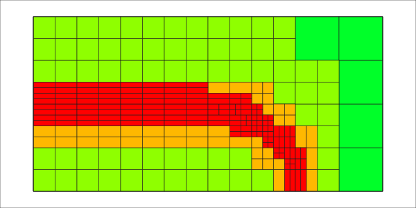
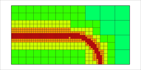
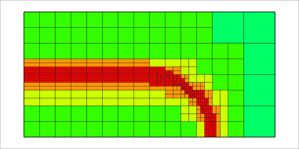
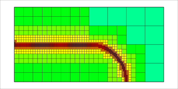
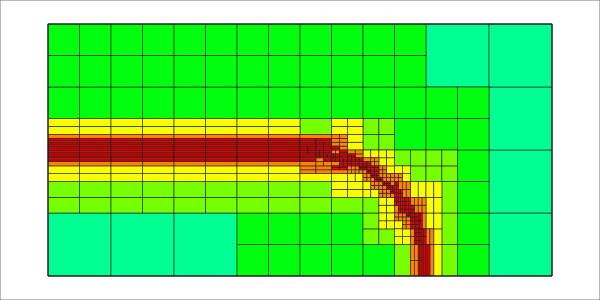
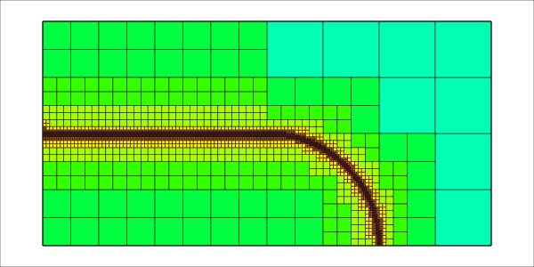
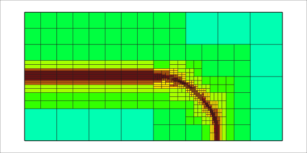
The first interesting part is of course to see how the meshes look like. On the left are the isotropically refined ones, on the right the anisotropic ones (colors indicate the refinement level of cells):
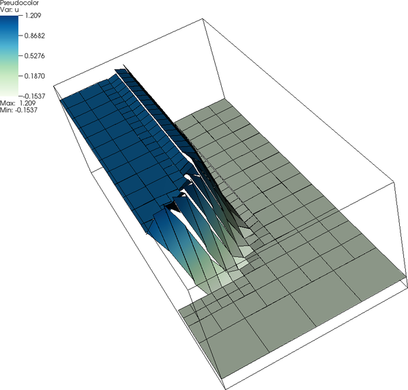
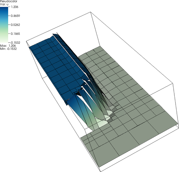
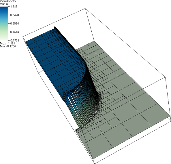
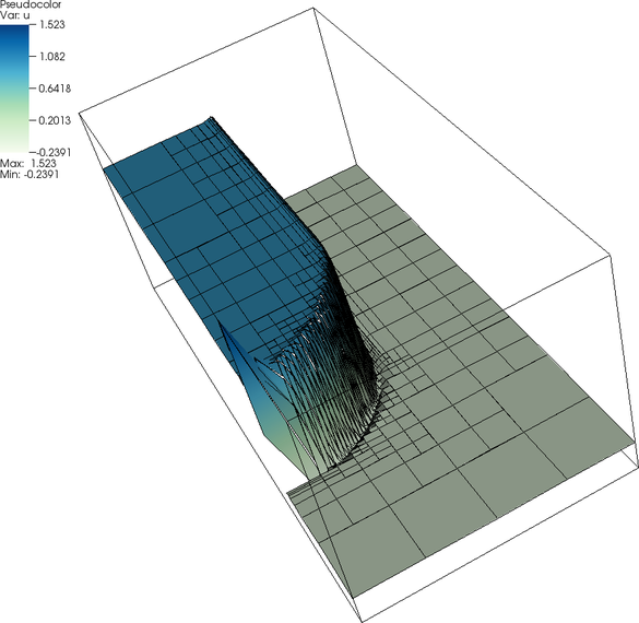
The other interesting thing is, of course, to see the solution on these two sequences of meshes. Here they are, on the refinement cycles 1 and 4, clearly showing that the solution is indeed composed of discontinuous piecewise polynomials:
We see, that the solution on the anisotropically refined mesh is very similar to the solution obtained on the isotropically refined mesh. Thus the anisotropic indicator seems to effectively select the appropriate cells for anisotropic refinement.
The pictures also explain why the mesh is refined as it is. In the whole left part of the domain refinement is only performed along the y-axis of cells. In the right part of the domain the refinement is dominated by isotropic refinement, as the anisotropic feature of the solution - the jump from one to zero - is not well aligned with the mesh where the advection direction takes a turn. However, at the bottom and closest (to the observer) parts of the quarter circle this jumps again becomes more and more aligned with the mesh and the refinement algorithm reacts by creating anisotropic cells of increasing aspect ratio.
It might seem that the necessary alignment of anisotropic features and the coarse mesh can decrease performance significantly for real world problems. That is not wrong in general: If one were, for example, to apply anisotropic refinement to problems in which shocks appear (e.g., the equations solved in step-69), then it many cases the shock is not aligned with the mesh and anisotropic refinement will help little unless one also introduces techniques to move the mesh in alignment with the shocks. On the other hand, many steep features of solutions are due to boundary layers. In those cases, the mesh is already aligned with the anisotropic features because it is of course aligned with the boundary itself, and anisotropic refinement will almost always increase the efficiency of computations on adapted grids for these cases.
The plain program
#include <array>
#include <iostream>
#include <fstream>
namespace Step30
{
template <int dim>
{
public:
virtual void value_list(
const std::vector<
Point<dim>> &points,
std::vector<double> &values,
const unsigned int = 0) const override
{
(void)points;
std::fill(values.begin(), values.end(), 0.);
}
};
template <int dim>
class BoundaryValues :
public Function<dim>
{
public:
virtual void value_list(
const std::vector<
Point<dim>> &points,
std::vector<double> &values,
const unsigned int = 0) const override
{
for (unsigned int i = 0; i < values.size(); ++i)
{
if (points[i][0] < 0.5)
values[i] = 1.;
else
values[i] = 0.;
}
}
};
template <int dim>
class Beta
{
public:
void value_list(
const std::vector<
Point<dim>> &points,
{
for (unsigned int i = 0; i < points.size(); ++i)
{
if (points[i][0] > 0)
{
values[i][0] = -points[i][1];
values[i][1] = points[i][0];
}
else
{
values[i][0] = -points[i][1];
}
}
}
};
template <int dim>
class DGTransportEquation
{
public:
DGTransportEquation();
private:
const Beta<dim> beta_function;
const RHS<dim> rhs_function;
const BoundaryValues<dim> boundary_function;
};
template <int dim>
DGTransportEquation<dim>::DGTransportEquation()
: beta_function()
, rhs_function()
, boundary_function()
{}
template <int dim>
void DGTransportEquation<dim>::assemble_cell_term(
{
{
cell_vector(i) +=
}
}
template <int dim>
void DGTransportEquation<dim>::assemble_boundary_term(
{
{
const double beta_n = beta[
point] * normals[
point];
if (beta_n > 0)
ui_vi_matrix(i, j) += beta_n * fe_v.
shape_value(j, point) *
else
cell_vector(i) -=
}
}
template <int dim>
void DGTransportEquation<dim>::assemble_face_term(
{
{
const double beta_n = beta[
point] * normals[
point];
if (beta_n > 0)
{
ui_vi_matrix(i, j) += beta_n * fe_v.
shape_value(j, point) *
ui_ve_matrix(k, j) -= beta_n * fe_v.
shape_value(j, point) *
}
else
{
ue_vi_matrix(i, l) += beta_n *
ue_ve_matrix(k, l) -=
}
}
}
template <int dim>
class DGMethod
{
public:
DGMethod(const bool anisotropic);
private:
void setup_system();
void assemble_system();
void refine_grid();
void set_anisotropic_flags();
void output_results(const unsigned int cycle) const;
const unsigned int degree;
const double anisotropic_threshold_ratio;
const bool anisotropic;
const QGauss<dim - 1> face_quadrature;
const DGTransportEquation<dim> dg;
};
template <int dim>
DGMethod<dim>::DGMethod(const bool anisotropic)
: mapping()
,
degree(1)
, fe(degree)
, anisotropic_threshold_ratio(3.)
, anisotropic(anisotropic)
,
quadrature(degree + 1)
, face_quadrature(degree + 1)
, dg()
{}
template <int dim>
void DGMethod<dim>::setup_system()
{
dof_handler.distribute_dofs(fe);
sparsity_pattern.reinit(dof_handler.n_dofs(),
dof_handler.n_dofs(),
1) *
fe.n_dofs_per_cell());
sparsity_pattern.compress();
system_matrix.reinit(sparsity_pattern);
solution2.reinit(dof_handler.n_dofs());
right_hand_side.reinit(dof_handler.n_dofs());
}
template <int dim>
void DGMethod<dim>::assemble_system()
{
const unsigned int dofs_per_cell = dof_handler.get_fe().n_dofs_per_cell();
std::vector<types::global_dof_index> dofs(dofs_per_cell);
std::vector<types::global_dof_index> dofs_neighbor(dofs_per_cell);
fe,
face_quadrature,
face_update_flags);
fe,
face_quadrature,
face_update_flags);
fe,
face_quadrature,
neighbor_face_update_flags);
for (const auto &cell : dof_handler.active_cell_iterators())
{
ui_vi_matrix = 0;
cell_vector = 0;
fe_v.reinit(cell);
dg.assemble_cell_term(fe_v, ui_vi_matrix, cell_vector);
cell->get_dof_indices(dofs);
for (const auto face_no : cell->face_indices())
{
const auto face = cell->face(face_no);
if (face->at_boundary())
{
fe_v_face.reinit(cell, face_no);
dg.assemble_boundary_term(fe_v_face, ui_vi_matrix, cell_vector);
}
else
{
ExcInternalError());
const auto neighbor = cell->neighbor(face_no);
if (face->has_children())
{
const unsigned int neighbor2 =
cell->neighbor_face_no(face_no);
for (unsigned int subface_no = 0;
subface_no < face->n_active_descendants();
++subface_no)
{
const auto neighbor_child =
cell->neighbor_child_on_subface(face_no, subface_no);
Assert(!neighbor_child->has_children(),
ExcInternalError());
ue_vi_matrix = 0;
ui_ve_matrix = 0;
ue_ve_matrix = 0;
fe_v_subface.reinit(cell, face_no, subface_no);
fe_v_face_neighbor.reinit(neighbor_child, neighbor2);
dg.assemble_face_term(fe_v_subface,
fe_v_face_neighbor,
ui_vi_matrix,
ue_vi_matrix,
ui_ve_matrix,
ue_ve_matrix);
neighbor_child->get_dof_indices(dofs_neighbor);
for (unsigned int i = 0; i < dofs_per_cell; ++i)
for (unsigned int j = 0; j < dofs_per_cell; ++j)
{
system_matrix.
add(dofs[i],
dofs_neighbor[j],
ue_vi_matrix(i, j));
system_matrix.add(dofs_neighbor[i],
dofs[j],
ui_ve_matrix(i, j));
system_matrix.add(dofs_neighbor[i],
dofs_neighbor[j],
ue_ve_matrix(i, j));
}
}
}
else
{
if (dim > 1 && cell->neighbor_is_coarser(face_no))
continue;
if (((dim > 1) && (cell->index() < neighbor->index())) ||
((dim == 1) && ((cell->level() < neighbor->level()) ||
((cell->level() == neighbor->level()) &&
(cell->index() < neighbor->index())))))
{
const unsigned int neighbor2 =
cell->neighbor_of_neighbor(face_no);
ue_vi_matrix = 0;
ui_ve_matrix = 0;
ue_ve_matrix = 0;
fe_v_face.reinit(cell, face_no);
fe_v_face_neighbor.reinit(neighbor, neighbor2);
dg.assemble_face_term(fe_v_face,
fe_v_face_neighbor,
ui_vi_matrix,
ue_vi_matrix,
ui_ve_matrix,
ue_ve_matrix);
neighbor->get_dof_indices(dofs_neighbor);
for (unsigned int i = 0; i < dofs_per_cell; ++i)
for (unsigned int j = 0; j < dofs_per_cell; ++j)
{
system_matrix.
add(dofs[i],
dofs_neighbor[j],
ue_vi_matrix(i, j));
system_matrix.add(dofs_neighbor[i],
dofs[j],
ui_ve_matrix(i, j));
system_matrix.add(dofs_neighbor[i],
dofs_neighbor[j],
ue_ve_matrix(i, j));
}
}
}
}
}
for (unsigned int i = 0; i < dofs_per_cell; ++i)
for (unsigned int j = 0; j < dofs_per_cell; ++j)
system_matrix.add(dofs[i], dofs[j], ui_vi_matrix(i, j));
for (unsigned int i = 0; i < dofs_per_cell; ++i)
right_hand_side(dofs[i]) += cell_vector(i);
}
}
template <int dim>
{
preconditioner.
initialize(system_matrix, fe.n_dofs_per_cell());
solver.solve(system_matrix, solution, right_hand_side, preconditioner);
}
template <int dim>
void DGMethod<dim>::refine_grid()
{
dof_handler,
solution2,
gradient_indicator);
gradient_indicator[cell->active_cell_index()] *=
gradient_indicator,
0.3,
0.1);
if (anisotropic)
set_anisotropic_flags();
}
template <int dim>
void DGMethod<dim>::set_anisotropic_flags()
{
fe,
face_quadrature,
face_update_flags);
fe,
face_quadrature,
face_update_flags);
fe,
face_quadrature,
for (const auto &cell : dof_handler.active_cell_iterators())
if (cell->refine_flag_set())
{
std::array<double, dim> jump_in_coordinate_direction;
std::array<double, dim> face_area_in_coordinate_direction;
for (const auto face_no : cell->face_indices())
{
const auto face = cell->face(face_no);
if (!face->at_boundary())
{
Assert(cell->neighbor(face_no).state() ==
ExcInternalError());
const auto neighbor = cell->neighbor(face_no);
std::vector<double> u(fe_v_face.n_quadrature_points);
std::vector<double> u_neighbor(fe_v_face.n_quadrature_points);
if (face->has_children())
{
unsigned int neighbor2 = cell->neighbor_face_no(face_no);
for (unsigned int subface_no = 0;
subface_no < face->n_active_descendants();
++subface_no)
{
const auto neighbor_child =
cell->neighbor_child_on_subface(face_no,
subface_no);
Assert(!neighbor_child->has_children(),
ExcInternalError());
fe_v_subface.reinit(cell, face_no, subface_no);
fe_v_face_neighbor.reinit(neighbor_child, neighbor2);
fe_v_subface.get_function_values(solution2, u);
fe_v_face_neighbor.get_function_values(solution2,
u_neighbor);
const std::vector<double> &JxW =
fe_v_subface.get_JxW_values();
for (unsigned int x = 0;
x < fe_v_subface.n_quadrature_points;
++x)
{
jump_in_coordinate_direction[face_no / 2] +=
std::abs(u[x] - u_neighbor[x]) * JxW[x];
face_area_in_coordinate_direction[face_no / 2] +=
JxW[x];
}
}
}
else
{
if (!cell->neighbor_is_coarser(face_no))
{
unsigned int neighbor2 =
cell->neighbor_of_neighbor(face_no);
fe_v_face.reinit(cell, face_no);
fe_v_face_neighbor.reinit(neighbor, neighbor2);
fe_v_face.get_function_values(solution2, u);
fe_v_face_neighbor.get_function_values(solution2,
u_neighbor);
const std::vector<double> &JxW =
fe_v_face.get_JxW_values();
for (unsigned int x = 0;
x < fe_v_face.n_quadrature_points;
++x)
{
jump_in_coordinate_direction[face_no / 2] +=
std::abs(u[x] - u_neighbor[x]) * JxW[x];
face_area_in_coordinate_direction[face_no / 2] +=
JxW[x];
}
}
else
{
std::pair<unsigned int, unsigned int>
neighbor_face_subface =
cell->neighbor_of_coarser_neighbor(face_no);
Assert(neighbor_face_subface.first < cell->n_faces(),
ExcInternalError());
Assert(neighbor_face_subface.second <
neighbor->face(neighbor_face_subface.first)
->n_active_descendants(),
ExcInternalError());
Assert(neighbor->neighbor_child_on_subface(
neighbor_face_subface.first,
neighbor_face_subface.second) == cell,
ExcInternalError());
fe_v_face.reinit(cell, face_no);
fe_v_subface.reinit(neighbor,
neighbor_face_subface.first,
neighbor_face_subface.second);
fe_v_face.get_function_values(solution2, u);
fe_v_subface.get_function_values(solution2,
u_neighbor);
const std::vector<double> &JxW =
fe_v_face.get_JxW_values();
for (unsigned int x = 0;
x < fe_v_face.n_quadrature_points;
++x)
{
jump_in_coordinate_direction[face_no / 2] +=
std::abs(u[x] - u_neighbor[x]) * JxW[x];
face_area_in_coordinate_direction[face_no / 2] +=
JxW[x];
}
}
}
}
}
std::array<double, dim> average_jumps;
double sum_of_average_jumps = 0.;
for (unsigned int i = 0; i < dim; ++i)
{
average_jumps[i] = jump_in_coordinate_direction[i] /
face_area_in_coordinate_direction[i];
sum_of_average_jumps += average_jumps[i];
}
for (unsigned int i = 0; i < dim; ++i)
if (average_jumps[i] > anisotropic_threshold_ratio *
(sum_of_average_jumps - average_jumps[i]))
}
}
template <int dim>
void DGMethod<dim>::output_results(const unsigned int cycle) const
{
std::string refine_type;
if (anisotropic)
refine_type = ".aniso";
else
refine_type = ".iso";
{
const std::string filename =
"grid-" + std::to_string(cycle) + refine_type + ".svg";
std::cout << " Writing grid to <" << filename << ">..." << std::endl;
std::ofstream svg_output(filename);
}
{
const std::string filename =
"sol-" + std::to_string(cycle) + refine_type + ".vtu";
std::cout << " Writing solution to <" << filename << ">..."
<< std::endl;
std::ofstream gnuplot_output(filename);
}
}
template <int dim>
void DGMethod<dim>::run()
{
for (unsigned int cycle = 0; cycle < 6; ++cycle)
{
std::cout << "Cycle " << cycle << ':' << std::endl;
if (cycle == 0)
{
p1[0] = -1.;
for (unsigned int i = 0; i < dim; ++i)
p2[i] = 1.;
std::vector<unsigned int> repetitions(dim, 1);
repetitions[0] = 2;
repetitions,
p1,
p2);
}
else
refine_grid();
std::cout << " Number of active cells: "
setup_system();
std::cout << " Number of degrees of freedom: " << dof_handler.n_dofs()
<< std::endl;
assemble_system();
std::cout <<
" Time of assemble_system: " << assemble_timer.
cpu_time()
<< std::endl;
solve(solution2);
output_results(cycle);
std::cout << std::endl;
}
}
}
int main()
{
try
{
using namespace Step30;
const unsigned int dim = 2;
{
std::cout << "Performing a " << dim
<< "D run with isotropic refinement..." << std::endl
<< "------------------------------------------------"
<< std::endl;
DGMethod<dim> dgmethod_iso(false);
dgmethod_iso.run();
}
{
std::cout << std::endl
<< "Performing a " << dim
<< "D run with anisotropic refinement..." << std::endl
<< "--------------------------------------------------"
<< std::endl;
DGMethod<dim> dgmethod_aniso(true);
dgmethod_aniso.run();
}
}
catch (std::exception &exc)
{
std::cerr << std::endl
<< std::endl
<< "----------------------------------------------------"
<< std::endl;
std::cerr << "Exception on processing: " << std::endl
<< exc.what() << std::endl
<< "Aborting!" << std::endl
<< "----------------------------------------------------"
<< std::endl;
return 1;
}
catch (...)
{
std::cerr << std::endl
<< std::endl
<< "----------------------------------------------------"
<< std::endl;
std::cerr << "Unknown exception!" << std::endl
<< "Aborting!" << std::endl
<< "----------------------------------------------------"
<< std::endl;
return 1;
};
return 0;
}
void write_vtu(std::ostream &out) const
void add_data_vector(const VectorType &data, const std::vector< std::string > &names, const DataVectorType type=type_automatic, const std::vector< DataComponentInterpretation::DataComponentInterpretation > &data_component_interpretation={})
virtual void build_patches(const unsigned int n_subdivisions=0)
const std::vector< double > & get_JxW_values() const
const std::vector< Point< spacedim > > & get_quadrature_points() const
const unsigned int dofs_per_cell
const unsigned int n_quadrature_points
const std::vector< Tensor< 1, spacedim > > & get_normal_vectors() const
const Tensor< 1, spacedim > & shape_grad(const unsigned int i, const unsigned int q_point) const
const double & shape_value(const unsigned int i, const unsigned int q_point) const
void add(const number a, const FullMatrix< number2 > &A)
void run(const Iterator &begin, const std_cxx20::type_identity_t< Iterator > &end, Worker worker, Copier copier, const ScratchData &sample_scratch_data, const CopyData &sample_copy_data, const unsigned int queue_length, const unsigned int chunk_size)
::VectorizedArray< Number, width > pow(const ::VectorizedArray< Number, width > &, const Number p)


