The 'Information density-based mesh refinement' code gallery program

This program was contributed by Wolfgang Bangerth <bangerth@colostate.edu>.
It comes without any warranty or support by its authors or the authors of deal.II.

This program is part of the deal.II code gallery and consists of the following files (click to inspect):

• Readme.md (annotated version)
• CMakeLists.txt
• doc/adjoint.png
• doc/entry-name
• doc/recovered-forward-solution.png
• doc/recovered-parameter.png
• doc/synthetic.png
• mesh_refinement.cc (annotated version)

Pictures from this code gallery program

Annotated version of Readme.md

Readme file for "Information density-based mesh refinement"

Note

This program implements the ideas and algorithms described in the paper "Estimating and using information in inverse problems" by Wolfgang Bangerth, Chris R. Johnson, Dennis K. Njeru, and Bart van Bloemen Waanders, 2022. See there for more information.

Motivation

Inverse problems are problems where we would like to infer properties of a system from measurements of the system's state or response to external stimuli. The specific example this program addresses is that we want to identify the source term (i.e., right hand side function) in an advection-diffusion equation from point measurements of the solution of the equation. A typical application is that we would like to find out the locations and strengths of pollution sources based on measuring the concentration of the polluting substance at a number of points.

It is clear that in order to solve such problems, one needs to "know" something about the system's state (here: the pollution concentration) through measurements. Intuitively, it is also clear that we know "more" about the pollution sources by (i) measuring at more points, and (ii) by measuring downstream from the sources than we would if we had measured upstream. Intuitive concepts such as this motivate wondering whether we can define an "information density" function whose value at a point \(\mathbf x\) describes how much we know about potential sources located at \(\mathbf x\).

The paper which this code accompanies explores the concept of information in inverse problems. It defines an "information density" by solving auxiliary problems for each measurement, and then outlines possible applications for these information densities in three vignettes: spatially variable regularization; mesh refinement; and optimal experimental design. It then considers one of these in detail through numerical experiments, namely mesh refinement. This program implements the algorithms shown there and produces the numerical results.

To run the code

After running cmake and compiling via make (or, if you have used the -G ... option of cmake, compiling the program via your favorite integrated development environment), you can run the executable by either just saying make run or using ./mesh_refinement on the command line. The default is to compile in "debug mode"; you can switch to "release mode" by saying make release and then compiling everything again.

The program contains a switch that decides which mesh refinement algorithm to use. By default, it refines the mesh based on the information criterion discussed in the paper; it runs a sequence of 7 mesh refinement cycles. In debug mode, running the program as is takes about 50 CPU minutes on a reasonably modern laptop. (The program takes about five and a half minutes in release mode.) It parallelizes certain operations, so the actual run time may be shorter depending on how many cores are available.

For each cycle, it outputs the solution as a VTU file, along with the \(A\), \(B\), \(C\), and \(M\) matrices discussed in the paper. These matrices can then be used to compute the eigenvalues of the \(H\) matrix defined by \(H = B^T A^{-T} C A^{-1} B + \beta M\) where \(\beta\) is the regularization parameters.

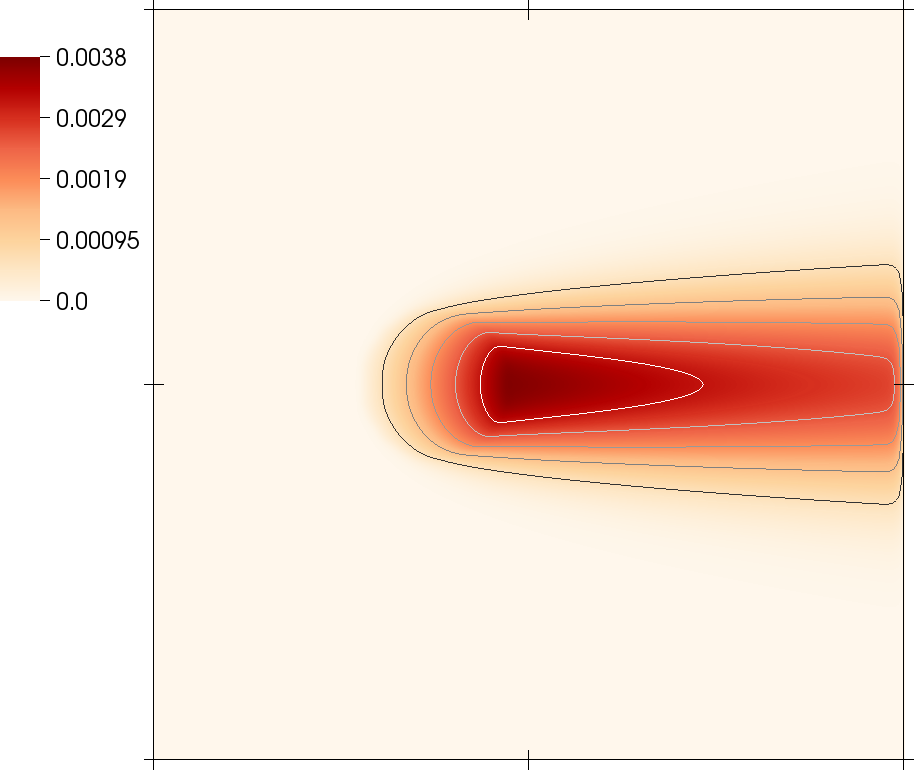
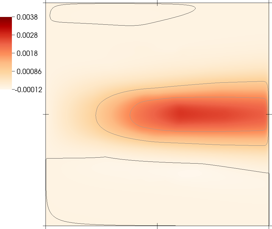
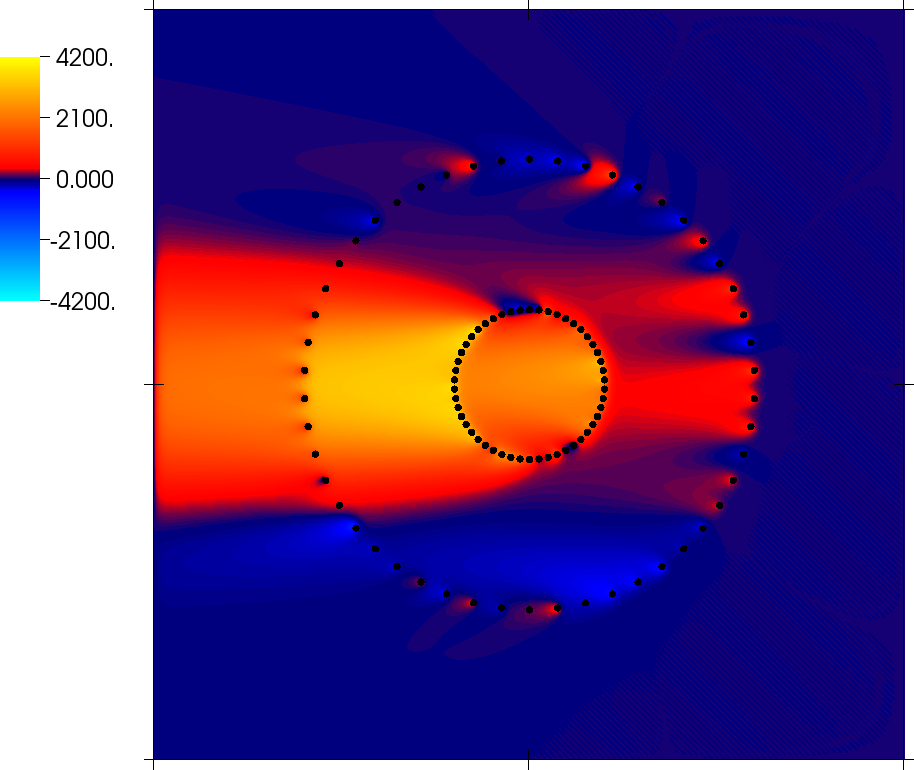
Some of the pictures shown in the paper are also reproduced as part of this code gallery program. See the paper for captions and more information.

Annotated version of mesh_refinement.cc

  /* ---------------------------------------------------------------------
   *
   * Copyright (C) 2022 by the deal.II authors and Wolfgang Bangerth.
   *
   * This file is part of the deal.II library.
   *
   * The deal.II library is free software; you can use it, redistribute
   * it, and/or modify it under the terms of the GNU Lesser General
   * Public License as published by the Free Software Foundation; either
   * version 2.1 of the License, or (at your option) any later version.
   * The full text of the license can be found in the file LICENSE.md at
   * the top level directory of deal.II.
   *
   * ---------------------------------------------------------------------
* 
   *
   * Author: Wolfgang Bangerth, Colorado State University, 2022.
   */
  
  
  #include <deal.II/base/numbers.h>
  #include <deal.II/grid/tria.h>
  #include <deal.II/dofs/dof_handler.h>
  #include <deal.II/grid/grid_generator.h>
  #include <deal.II/grid/tria_accessor.h>
  #include <deal.II/grid/tria_iterator.h>
  #include <deal.II/dofs/dof_accessor.h>
  #include <deal.II/dofs/dof_renumbering.h>
  #include <deal.II/fe/fe_q.h>
  #include <deal.II/fe/fe_dgq.h>
  #include <deal.II/fe/fe_system.h>
  #include <deal.II/dofs/dof_tools.h>
  #include <deal.II/fe/fe_values.h>
  #include <deal.II/base/quadrature_lib.h>
  #include <deal.II/base/function.h>
  #include <deal.II/numerics/vector_tools.h>
  #include <deal.II/numerics/matrix_tools.h>
  #include <deal.II/numerics/derivative_approximation.h>
  #include <deal.II/lac/block_vector.h>
  #include <deal.II/lac/full_matrix.h>
  #include <deal.II/lac/block_sparse_matrix.h>
  #include <deal.II/lac/block_sparsity_pattern.h>
  #include <deal.II/lac/sparse_direct.h>
  #include <deal.II/particles/particle_handler.h>
  #include <deal.II/particles/data_out.h>
  
  #include <deal.II/numerics/data_out.h>
  #include <fstream>
  #include <iostream>
  
  #include <deal.II/base/logstream.h>
  #include <deal.II/grid/grid_refinement.h>
  
  using namespace dealii;

The following is the main class. It resembles a variation of the step-6 principal class, with the addition of information-specific stuff. It also has to deal with solving a vector-valued problem for (c,lambda,f) as primal variable, dual variable, and right hand side, as explained in the paper.

template <int dim>
class InformationDensityMeshRefinement
{
public:
  InformationDensityMeshRefinement ();
  void run ();
 
private:
  void compute_synthetic_measurements();
  void bounce_measurement_points_to_cell_centers ();
  void setup_system();
  void assemble_system ();
  void solve ();
  void compute_information_content ();
  void output_results (const unsigned int cycle) const;
  void refine_grid ();
 
  const Point<dim>          source_location;
  const double              source_radius;
 
  std::vector<Point<dim>>   detector_locations;
  
  const double              regularization_parameter;
  Tensor<1,dim>             velocity;
 
  Triangulation<dim>        triangulation;
  FESystem<dim>             fe;
  DoFHandler<dim>           dof_handler;
 
  AffineConstraints<double> hanging_node_constraints;
 
  BlockSparsityPattern      sparsity_pattern;
  BlockSparseMatrix<double> system_matrix;
 
  BlockVector<double>       solution;
  BlockVector<double>       system_rhs;
 
  Vector<double>            information_content;
 
  std::vector<Point<dim>>   detector_locations_on_mesh;
  std::vector<double>       measurement_values;
  std::vector<double>       noise_level;
};
 
 
 
 
template <int dim>
InformationDensityMeshRefinement<dim>::InformationDensityMeshRefinement ()
:
source_location (Point<dim>(-0.25,0)),
source_radius (0.2),
regularization_parameter (10000),
fe (FE_Q<dim>(3), 1,    // c
    FE_Q<dim>(3), 1,    // lambda
    FE_DGQ<dim>(0), 1), // f
dof_handler (triangulation)
{
  velocity[0] = 100;

We have 50 detector points on an outer ring...

for (unsigned int i=0; i<50; ++i)
  {
    const Point<dim> p (0.6 * std::sin(2*numbers::PI * i/50),
                        0.6 * std::cos(2*numbers::PI * i/50));
    detector_locations.push_back (p);
  }

...and another 50 detector points on an innner ring:

for (unsigned int i=0; i<50; ++i)
  {
    const Point<dim> p (0.2 * std::sin(2*numbers::PI * i/50),
                        0.2 * std::cos(2*numbers::PI * i/50));
    detector_locations.push_back (p);
  }

Generate the grid we will work on:

GridGenerator::hyper_cube (triangulation, -1, 1);
triangulation.refine_global (4);

The detector locations are static, so we can already here generate a file that contains their locations. We use the particle framework to do this, using detector locations as particle locations.

{
  Particles::ParticleHandler<dim> particle_handler(triangulation,
                                                   StaticMappingQ1<dim>::mapping);
  for (const auto &loc : detector_locations)
    {
      Particles::Particle<dim> new_particle;
      new_particle.set_location(loc);

Insert the particle. It is a lie that the particle is in the first cell, but nothing we do actually cares about the cell a particle is in.

      particle_handler.insert_particle(new_particle,
                                       triangulation.begin_active());
    }
 
  Particles::DataOut<dim> particle_out;
  particle_out.build_patches(particle_handler);
  std::ofstream output("detector_locations.vtu");
  particle_out.write_vtu(output);
}

While we're generating output, also output the source location. Do this by outputting many (1000) points that indicate the perimeter of the source

  {
    Particles::ParticleHandler<dim> particle_handler(triangulation,
                                                     StaticMappingQ1<dim>::mapping);
 
    const unsigned int n_points = 1000;
    for (unsigned int i=0; i<n_points; ++i)
      {
        Point<dim> loc = source_location;
        loc[0] += source_radius * std::cos(2*numbers::PI*i/n_points);
        loc[1] += source_radius * std::sin(2*numbers::PI*i/n_points);
        
        Particles::Particle<dim> new_particle;
        new_particle.set_location(loc);
        particle_handler.insert_particle(new_particle,
                                         triangulation.begin_active());
      }
    
    Particles::DataOut<dim> particle_out;
    particle_out.build_patches(particle_handler);
    std::ofstream output("source_locations.vtu");
    particle_out.write_vtu(output);
  }
}

The following function solves a forward problem on a twice refined mesh to compute "synthetic data". Refining the mesh beyond the mesh used for the inverse problem avoids an inverse crime.

template <int dim>
void InformationDensityMeshRefinement<dim>::compute_synthetic_measurements ()
{
  std::cout << "Computing synthetic data by solving the forward problem..."
            << std::flush;

Create a triangulation and DoFHandler that corresponds to a twice-refined mesh so that we obtain the synthetic data with higher accuracy than we do on the regular mesh used for all other computations.

Triangulation<dim> forward_triangulation;
forward_triangulation.copy_triangulation (triangulation);
forward_triangulation.refine_global (2);
 
const FE_Q<dim> forward_fe (fe.base_element(0).degree);
DoFHandler<dim> forward_dof_handler (forward_triangulation);
forward_dof_handler.distribute_dofs (forward_fe);
 
AffineConstraints<double> constraints;
DoFTools::make_hanging_node_constraints(forward_dof_handler, constraints);
constraints.close();
 
SparsityPattern sparsity (forward_dof_handler.n_dofs(),
                          forward_dof_handler.max_couplings_between_dofs());
DoFTools::make_sparsity_pattern (forward_dof_handler, sparsity);
constraints.condense (sparsity);
sparsity.compress ();
 
SparseMatrix<double> system_matrix (sparsity);
Vector<double>       system_rhs (forward_dof_handler.n_dofs());
 
QGauss<dim>  quadrature_formula(3);
FEValues<dim> fe_values (forward_fe, quadrature_formula,
                         update_values   | update_gradients |
                         update_quadrature_points | update_JxW_values);
 
const unsigned int   dofs_per_cell = forward_fe.dofs_per_cell;
const unsigned int   n_q_points    = quadrature_formula.size();

First assemble the system matrix and right hand side for the forward problem:

{
  FullMatrix<double>   cell_matrix (dofs_per_cell, dofs_per_cell);
  Vector<double>       cell_rhs (dofs_per_cell);
  std::vector<unsigned int> local_dof_indices (dofs_per_cell);
 
  for (const auto &cell : forward_dof_handler.active_cell_iterators())
    {
      fe_values.reinit (cell);
      cell_matrix = 0;
      cell_rhs = 0;
 
      for (unsigned int q_point=0; q_point<n_q_points; ++q_point)
        for (unsigned int i=0; i<dofs_per_cell; ++i)
          for (unsigned int j=0; j<dofs_per_cell; ++j)
            cell_matrix(i,j) += (fe_values.shape_grad(i,q_point) *
                                 fe_values.shape_grad(j,q_point)
                                 +
                                 fe_values.shape_value(i,q_point) *
                                 (velocity * fe_values.shape_grad(j,q_point))
            )
                                *
                                fe_values.JxW(q_point);
      for (unsigned int q_point=0; q_point<n_q_points; ++q_point)
        if (fe_values.quadrature_point(q_point).distance (source_location)
            < source_radius)
          for (unsigned int i=0; i<dofs_per_cell; ++i)
            cell_rhs(i) +=
              1.0 *
              fe_values.shape_value (i, q_point) *
              fe_values.JxW(q_point);
 
      cell->get_dof_indices (local_dof_indices);
      constraints.distribute_local_to_global (cell_matrix,
                                              cell_rhs,
                                              local_dof_indices,
                                              system_matrix,
                                              system_rhs);
    }
 
  std::map<unsigned int, double> boundary_values;
  VectorTools::interpolate_boundary_values (forward_dof_handler,
                                            0,
                                            Functions::ZeroFunction<dim>(),
                                            boundary_values);
  Vector<double> tmp (forward_dof_handler.n_dofs());
  MatrixTools::apply_boundary_values (boundary_values,
                                      system_matrix,
                                      tmp,
                                      system_rhs);
}

Solve the forward problem and output it into its own VTU file :

SparseDirectUMFPACK A_inverse;
Vector<double> forward_solution (forward_dof_handler.n_dofs());
forward_solution = system_rhs;
A_inverse.solve(system_matrix, forward_solution);
 
const double max_forward_solution = forward_solution.linfty_norm();
 
{
  DataOut<dim> data_out;
  data_out.attach_dof_handler (forward_dof_handler);
  data_out.add_data_vector (forward_solution, "c");
  data_out.build_patches (4);
 
  std::ofstream out ("forward-solution.vtu");
  data_out.write_vtu (out);
}

Now evaluate the forward solution at the measurement points:

for (const auto &p : detector_locations)
  {

same 10% noise level for all points

      noise_level.push_back (0.1 * max_forward_solution);
 
      const double z_n = VectorTools::point_value(forward_dof_handler, forward_solution, p);
      const double eps_n = Utilities::generate_normal_random_number(0, noise_level.back());
 
      measurement_values.push_back (z_n + eps_n);
    }
 
  std::cout << std::endl;
}

It will make our lives easier if we can always assume that detector locations are at cell centers, because then we can evaluate the solution there using a quadrature formula whose sole quadrature point lies at the center of a cell. That's of course not where the "real" detector locations are, but it does not introduce a large error to do this.

template <int dim>
void InformationDensityMeshRefinement<dim>::bounce_measurement_points_to_cell_centers ()
{
  detector_locations_on_mesh = detector_locations;
  for (auto &p : detector_locations_on_mesh)
    {
      for (const auto &cell : triangulation.active_cell_iterators())
        if (cell->point_inside (p))
          {
            p =  cell->center();
            break;
          }
    }
}

The following functions are all quite standard by what we have shown in step-4, step-6, and step-22 (to name just a few of the more typical programs):

template <int dim>
void InformationDensityMeshRefinement<dim>::setup_system ()
{
  std::cout << "Setting up the linear system for the inverse problem..."
            << std::endl;
  
  dof_handler.distribute_dofs (fe);
  DoFRenumbering::component_wise (dof_handler);
 
  hanging_node_constraints.clear ();
  DoFTools::make_hanging_node_constraints(dof_handler,
                                          hanging_node_constraints);
  hanging_node_constraints.close();
 
  std::cout << "   Number of active cells: "
            << triangulation.n_active_cells()
            << std::endl;
  std::cout << "   Number of degrees of freedom: "
            << dof_handler.n_dofs()
            << std::endl;
 
  const std::vector<types::global_dof_index> dofs_per_component =
    DoFTools::count_dofs_per_fe_component(dof_handler);
  BlockDynamicSparsityPattern c_sparsity(dofs_per_component,dofs_per_component);
  DoFTools::make_sparsity_pattern (dof_handler, c_sparsity);
  hanging_node_constraints.condense(c_sparsity);
  sparsity_pattern.copy_from(c_sparsity);
 
  system_matrix.reinit (sparsity_pattern);
 
  solution.reinit (dofs_per_component);
  system_rhs.reinit (dofs_per_component);
}
 
 
 
template <int dim>
void InformationDensityMeshRefinement<dim>::assemble_system ()
{
  std::cout << "Assembling the linear system for the inverse problem..."
            << std::flush;
  
  QGauss<dim>  quadrature_formula(3);
 
  FEValues<dim> fe_values (fe, quadrature_formula,
                           update_values   | update_gradients |
                           update_quadrature_points | update_JxW_values);
 
  const unsigned int   dofs_per_cell = fe.dofs_per_cell;
  const unsigned int   n_q_points    = quadrature_formula.size();
 
  FullMatrix<double>   cell_matrix (dofs_per_cell, dofs_per_cell);
  Vector<double>       cell_rhs (dofs_per_cell);
 
  std::vector<unsigned int> local_dof_indices (dofs_per_cell);
 
  FEValuesExtractors::Scalar c(0), lambda(1), f(2);
 
  for (const auto &cell : dof_handler.active_cell_iterators())
    {
      fe_values.reinit (cell);
      cell_matrix = 0;
      cell_rhs = 0;
 
      for (unsigned int q_point=0; q_point<n_q_points; ++q_point)
        for (unsigned int i=0; i<dofs_per_cell; ++i)
          {
            const Tensor<1,dim> grad_phi_i = fe_values[c].gradient (i,q_point);
            const Tensor<1,dim> grad_psi_i = fe_values[lambda].gradient (i,q_point);
 
            const double phi_i = fe_values[c].value (i,q_point);
            const double psi_i = fe_values[lambda].value (i,q_point);
            const double chi_i = fe_values[f].value (i,q_point);
 
            for (unsigned int j=0; j<dofs_per_cell; ++j)
              {
                const Tensor<1,dim> grad_phi_j = fe_values[c].gradient (j,q_point);
                const Tensor<1,dim> grad_psi_j = fe_values[lambda].gradient (j,q_point);
 
                const double phi_j = fe_values[c].value (j,q_point);
                const double psi_j= fe_values[lambda].value (j,q_point);
                const double chi_j = fe_values[f].value (j,q_point);
 
                cell_matrix(i,j) +=
                  ((grad_phi_i * grad_phi_j
                    +
                    phi_i * (velocity * grad_phi_j)
                    -
                    phi_i * chi_j
                    +
                    grad_psi_i * grad_psi_j
                    -
                    psi_i * (velocity * grad_psi_j)
                    -
                    chi_i * psi_j
                    +
                    regularization_parameter * chi_i * chi_j
                  ) *
                   fe_values.JxW (q_point));
 
                for (unsigned int n=0; n< detector_locations_on_mesh.size(); ++n)
                  if (fe_values.quadrature_point(q_point).distance (detector_locations_on_mesh[n]) < 1e-12)
                    {
                      cell_matrix(i,j) += psi_i * phi_j / noise_level[n] / noise_level[n];
                    }
              }
 
            for (unsigned int n=0; n< detector_locations_on_mesh.size(); ++n)
              if (fe_values.quadrature_point(q_point).distance (detector_locations_on_mesh[n]) < 1e-12)
                cell_rhs(i) += psi_i * measurement_values[n] / noise_level[n] / noise_level[n];
          }
 
      cell->get_dof_indices (local_dof_indices);
      for (unsigned int i=0; i<dofs_per_cell; ++i)
        {
          for (unsigned int j=0; j<dofs_per_cell; ++j)
            system_matrix.add (local_dof_indices[i],
                               local_dof_indices[j],
                               cell_matrix(i,j));
 
          system_rhs(local_dof_indices[i]) += cell_rhs(i);
        }
    }
 
  hanging_node_constraints.condense (system_matrix);
  hanging_node_constraints.condense (system_rhs);
 
  std::map<unsigned int,double> boundary_values;
  std::vector<bool> component_mask (3);
  component_mask[0] = component_mask[1] = true;
  component_mask[2] = false;
  VectorTools::interpolate_boundary_values (dof_handler,
                                            0,
                                            Functions::ZeroFunction<dim>(3),
                                            boundary_values,
                                            component_mask);
  MatrixTools::apply_boundary_values (boundary_values,
                                      system_matrix,
                                      solution,
                                      system_rhs);
 
  std::cout << std::endl;
}
 
 
 
template <int dim>
void InformationDensityMeshRefinement<dim>::solve ()
{
  std::cout << "Solving the linear system for the inverse problem..."
            << std::flush;
  
  SparseDirectUMFPACK  A_direct;
  solution = system_rhs;
  A_direct.solve(system_matrix, solution);
 
  hanging_node_constraints.distribute (solution);
 
  std::cout << std::endl;
}

This is really the only interesting function of this program. It computes the functions \(h_K = A^{-1} s_K\) for each source function (corresponding to each cell of the mesh). To do so, it first computes the forward matrix \(A\) and uses the SparseDirectUMFPACK class to build an LU decomposition for this matrix. Then it loops over all cells \(K\) and computes the corresponding \(h_K\) by applying the LU decomposition to a right hand side vector for each \(s_K\).

The actual information content is then computed by evaluating these functions \(h_K\) at measurement locations.

template <int dim>
void InformationDensityMeshRefinement<dim>::compute_information_content ()
{
  std::cout << "Computing the information content..."
            << std::flush;
  
  information_content.reinit (triangulation.n_active_cells());
 
  const FE_Q<dim> information_fe (fe.base_element(0).degree);
  DoFHandler<dim> information_dof_handler (triangulation);
  information_dof_handler.distribute_dofs (information_fe);
 
  AffineConstraints<double> constraints;
  DoFTools::make_hanging_node_constraints(information_dof_handler, constraints);
  constraints.close();
 
  SparsityPattern sparsity (information_dof_handler.n_dofs(),
                            information_dof_handler.max_couplings_between_dofs());
  DoFTools::make_sparsity_pattern (information_dof_handler, sparsity);
  constraints.condense (sparsity);
  sparsity.compress ();
 
  SparseMatrix<double> system_matrix (sparsity);
 
  QGauss<dim>  quadrature_formula(3);
 
  const unsigned int   dofs_per_cell = information_fe.dofs_per_cell;
  const unsigned int   n_q_points    = quadrature_formula.size();

First build the forward operator

{
  FEValues<dim> fe_values (information_fe, quadrature_formula,
                           update_values   | update_gradients |
                           update_quadrature_points | update_JxW_values);
 
  FullMatrix<double>   cell_matrix (dofs_per_cell, dofs_per_cell);
  std::vector<unsigned int> local_dof_indices (dofs_per_cell);
 
  for (const auto &cell : information_dof_handler.active_cell_iterators())
    {
      fe_values.reinit (cell);
      cell_matrix = 0;
 
      for (unsigned int q_point=0; q_point<n_q_points; ++q_point)
        for (unsigned int i=0; i<dofs_per_cell; ++i)
          for (unsigned int j=0; j<dofs_per_cell; ++j)
            cell_matrix(i,j) += (fe_values.shape_grad (i,q_point) *
                                 fe_values.shape_grad(j,q_point)
                                 +
                                 fe_values.shape_value(i,q_point) *
                                 (velocity * fe_values.shape_grad(j,q_point))) *
                                fe_values.JxW(q_point);
 
      cell->distribute_local_to_global (cell_matrix,
                                        system_matrix);
    }
 
  constraints.condense (system_matrix);
 
  std::map<unsigned int, double> boundary_values;
  VectorTools::interpolate_boundary_values (information_dof_handler,
                                            0,
                                            Functions::ZeroFunction<dim>(),
                                            boundary_values);
  Vector<double> tmp (information_dof_handler.n_dofs());
  MatrixTools::apply_boundary_values (boundary_values,
                                      system_matrix,
                                      tmp,
                                      tmp);
}

Then factorize

SparseDirectUMFPACK A_inverse;
A_inverse.factorize(system_matrix);

Now compute the solutions corresponding to the possible sources. Each source is active on exactly one cell.

As mentioned in the paper, this is a trivially parallel job, so we send the computations for each of these cells onto a separate task and let the OS schedule them onto individual processor cores.

Threads::TaskGroup<void> tasks;
for (unsigned int K=0; K<triangulation.n_active_cells(); ++K)
  tasks +=
    Threads::new_task([&,K]()
                      {
                        Vector<double> rhs (information_dof_handler.n_dofs());
                        Vector<double> cell_rhs (dofs_per_cell);
                        std::vector<unsigned int> local_dof_indices (dofs_per_cell);
 
                        typename DoFHandler<dim>::active_cell_iterator
                          cell = information_dof_handler.begin_active();
                        std::advance (cell, K);
 
                        FEValues<dim> fe_values (information_fe, quadrature_formula,
                                                 update_values |
                                                 update_quadrature_points | update_JxW_values);
 
                        fe_values.reinit (cell);
                        cell_rhs = 0;
 
                        for (unsigned int q_point=0; q_point<n_q_points; ++q_point)
                          for (unsigned int i=0; i<dofs_per_cell; ++i)
                            cell_rhs(i) += fe_values.shape_value (i,q_point) *
                                           fe_values.JxW(q_point);
 
                        cell->distribute_local_to_global (cell_rhs,
                                                          rhs);
 
                        constraints.condense (rhs);
 
                        A_inverse.solve(rhs);
 
                        constraints.distribute (rhs);

Having computed the forward solutions corresponding to this source term, evaluate its contribution to the information content on all cells of the mesh by taking into account the detector locations. We add these into global objects, so we have to guard access to the global object:

                    static std::mutex m;
                    std::lock_guard<std::mutex> g(m);
             
 
                    information_content(K) = regularization_parameter * cell->measure() * cell->measure();
                    std::vector<double> local_h_K_values (n_q_points);
                    for (const auto &cell : information_dof_handler.active_cell_iterators())
                      {
                        fe_values.reinit (cell);
                        fe_values.get_function_values (rhs, local_h_K_values);
 
                        for (unsigned int q_point=0; q_point<n_q_points; ++q_point)
                          for (unsigned int n=0; n< detector_locations_on_mesh.size(); ++n)
                            if (fe_values.quadrature_point(q_point).distance (detector_locations_on_mesh[n]) < 1e-12)
                              information_content(K) += local_h_K_values[q_point]
                                                        * local_h_K_values[q_point]
                                                        / noise_level[n] / noise_level[n];
                      }
                  }
);

And wait:

  tasks.join_all();
 
  std::cout << std::endl;
}

Create graphical output for all of the principal variables of the problem (c,lambda,f) as well as for the information content and density. Then also output the various blocks of the matrix so we can compute the eigenvalues of the H matrix mentioned in the paper.

template <int dim>
void InformationDensityMeshRefinement<dim>::output_results (const unsigned int cycle) const
{
  std::cout << "Outputting solutions..." << std::flush;
  
  DataOut<dim> data_out;
 
  std::vector<std::string> names;
  names.push_back ("forward_solution");
  names.push_back ("adjoint_solution");
  names.push_back ("recovered_parameter");
 
  data_out.attach_dof_handler (dof_handler);
  data_out.add_data_vector (solution, names);
  data_out.add_data_vector (information_content, "information_content");
 
  Vector<double> information_density (triangulation.n_active_cells());
  for (const auto &cell : triangulation.active_cell_iterators())
    information_density(cell->active_cell_index())
      = std::sqrt(information_content(cell->active_cell_index())) / cell->measure();
  data_out.add_data_vector (information_density, "information_density");
 
  data_out.build_patches ();
 
  std::string filename = "solution-";
  filename += ('0'+cycle);
  filename += ".vtu";
 
  std::ofstream output (filename.c_str());
  data_out.write_vtu (output);

Now output the individual blocks of the matrix into files.

  auto write_block = [&](const unsigned int block_i,
                         const unsigned int block_j,
                         const std::string &filename)
                     {
                           std::ofstream o(filename);
                           system_matrix.block(block_i,block_j).print (o);
                     };
  write_block(0,0, "matrix-" + std::to_string(cycle) + "-A.txt");
  write_block(0,2, "matrix-" + std::to_string(cycle) + "-B.txt");
  write_block(1,0, "matrix-" + std::to_string(cycle) + "-C.txt");
  write_block(2,2, "matrix-" + std::to_string(cycle) + "-M.txt");  
  
  std::cout << std::endl;
}

The following is then a function that refines the mesh based on the refinement criteria described in the paper. Which criterion to use is determined by which value the refinement_criterion variable is set to.

template <int dim>
void InformationDensityMeshRefinement<dim>::refine_grid ()
{
  std::cout << "Refining the mesh..." << std::endl;
  
  enum RefinementCriterion
  {
        global,
        information_content,
        indicator,
        smoothness
  };
  const RefinementCriterion refinement_criterion = information_content;
 
  switch (refinement_criterion)
    {
    case global:
    {
      triangulation.refine_global();
      break;
    }
    
    case information_content:
    {
      GridRefinement::refine_and_coarsen_fixed_number(triangulation,
                                                      this->information_content,
                                                      0.2, 0.05);
      triangulation.execute_coarsening_and_refinement ();
      break;
    }
    
    case indicator:
    {
      Vector<double> refinement_indicators (triangulation.n_active_cells());
      
      QGauss<dim> quadrature(3);
      FEValues<dim> fe_values (fe, quadrature, update_values | update_JxW_values);
 
      FEValuesExtractors::Scalar lambda(1), f(2);
 
      std::vector<double> lambda_values (quadrature.size());
      std::vector<double> f_values (quadrature.size());
 
      for (const auto &cell : dof_handler.active_cell_iterators())
        {
          fe_values.reinit (cell);
          fe_values[lambda].get_function_values (solution, lambda_values);
          fe_values[f].get_function_values (solution, f_values);
 
          for (unsigned int q=0; q<quadrature.size(); ++q)
            refinement_indicators(cell->active_cell_index())
              += (std::fabs (regularization_parameter * f_values[q]
                             -
                             lambda_values[q])
                  * fe_values.JxW(q));
        }
 
      GridRefinement::refine_and_coarsen_fixed_number(triangulation,
                                                      refinement_indicators,
                                                      0.2, 0.05);
      triangulation.execute_coarsening_and_refinement ();
      break;
    }
    
    
    case smoothness:
    {
      Vector<float> refinement_indicators (triangulation.n_active_cells());
      
      DerivativeApproximation::approximate_gradient(dof_handler,
                                                    solution,
                                                    refinement_indicators,
                                                    /*component=*/2);

and scale it to obtain an error indicator.

      for (const auto &cell : triangulation.active_cell_iterators())
        refinement_indicators[cell->active_cell_index()] *=
          std::pow(cell->diameter(), 1 + 1.0 * dim / 2);
      
      
      GridRefinement::refine_and_coarsen_fixed_number(triangulation,
                                                      refinement_indicators,
                                                      0.2, 0.05);
      triangulation.execute_coarsening_and_refinement ();
      break;
    }
 
    default:
          Assert (false, ExcInternalError());
    }
  
  bounce_measurement_points_to_cell_centers ();
 
 
  std::cout << std::endl;
}
 
 
 
 
template <int dim>
void InformationDensityMeshRefinement<dim>::run ()
{
  std::cout << "Solving problem in " << dim << " space dimensions." << std::endl;
 
  compute_synthetic_measurements ();
  bounce_measurement_points_to_cell_centers ();
 
  for (unsigned int cycle=0; cycle<7; ++cycle)
    {
      std::cout << "---------- Cycle " << cycle << " ------------" << std::endl;
    
      setup_system ();
      assemble_system ();
      solve ();
      compute_information_content ();
      output_results (cycle);
      refine_grid ();
    }
}
 
 
 
int main ()
{
  try
    {
      deallog.depth_console (0);
 
      InformationDensityMeshRefinement<2> information_density_mesh_refinement;
      information_density_mesh_refinement.run ();
    }
  catch (std::exception &exc)
    {
      std::cerr << std::endl << std::endl
                << "----------------------------------------------------"
                << std::endl;
      std::cerr << "Exception on processing: " << std::endl
                << exc.what() << std::endl
                << "Aborting!" << std::endl
                << "----------------------------------------------------"
                << std::endl;
 
      return 1;
    }
  catch (...)
    {
      std::cerr << std::endl << std::endl
                << "----------------------------------------------------"
                << std::endl;
      std::cerr << "Unknown exception!" << std::endl
                << "Aborting!" << std::endl
                << "----------------------------------------------------"
                << std::endl;
      return 1;
    }
 
  return 0;
}