 |
Reference documentation for deal.II version 9.3.3
|
 |
Reference documentation for deal.II version 9.3.3
|
This tutorial depends on step-15.
| Table of contents | |
|---|---|
This program was contributed by Jörg Frohne (University of Siegen, Germany) while on a long-term visit to Texas A&M University.
This material is based upon work partly supported by ThyssenKrupp Steel Europe.
This example is based on the Laplace equation in 2d and deals with the question what happens if a membrane is deflected by some external force but is also constrained by an obstacle. In other words, think of a elastic membrane clamped at the boundary to a rectangular frame (we choose \Omega = \left[-1,1\right]^2) and that sags through due to gravity acting on it. What happens now if there is an obstacle under the membrane that prevents it from reaching its equilibrium position if gravity was the only existing force? In the current example program, we will consider that under the membrane is a stair step obstacle against which gravity pushes the membrane.
This problem is typically called the "obstacle problem" (see also this Wikipedia article), and it results in a variational inequality, rather than a variational equation when put into the weak form. We will below derive it from the classical formulation, but before we go on to discuss the mathematics let us show how the solution of the problem we will consider in this tutorial program looks to gain some intuition of what we should expect:
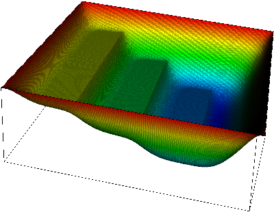 | 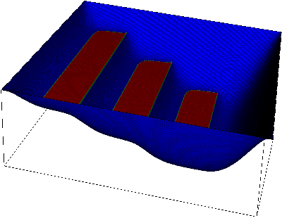 |
Here, at the left, we see the displacement of the membrane. The shape of the obstacle underneath is clearly visible. On the right, we overlay which parts of the membrane are in contact with the obstacle. We will later call this set of points the "active set" to indicate that an inequality constraint is active there.
The classical formulation of the problem possesses the following form:
\begin{align*} -\textrm{div}\ \sigma &\geq f & &\quad\text{in } \Omega,\\ \sigma &= \nabla u & &\quad\text{in } \Omega,\\ u(\mathbf x) &= 0 & &\quad\text{on }\partial\Omega,\\ (-\Delta u - f)(u - g) &= 0 & &\quad\text{in } \Omega,\\ u(\mathbf x) &\geq g(\mathbf x) & &\quad\text{in } \Omega \end{align*}
with u\in H^2(\Omega). u is a scalar valued function that denotes the vertical displacement of the membrane. The first equation is called equilibrium condition with a force of areal density f. Here, we will consider this force to be gravity. The second one is known as Hooke's Law that says that the stresses \sigma are proportional to the gradient of the displacements u (the proportionality constant, often denoted by E, has been set to one here, without loss of generality; if it is constant, it can be put into the right hand side function). At the boundary we have zero Dirichlet conditions. Obviously, the first two equations can be combined to yield -\Delta u \ge f.
Intuitively, gravity acts downward and so f(\mathbf x) is a negative function (we choose f=-10 in this program). The first condition then means that the total force acting on the membrane is gravity plus something positive: namely the upward force that the obstacle exerts on the membrane at those places where the two of them are in contact. How big is this additional force? We don't know yet (and neither do we know "where" it actually acts) but it must be so that the membrane doesn't penetrate the obstacle.
The fourth equality above together with the last inequality forms the obstacle condition which has to hold at every point of the whole domain. The latter of these two means that the membrane must be above the obstacle g(\mathbf x) everywhere. The second to last equation, often called the "complementarity condition" says that where the membrane is not in contact with the obstacle (i.e., those \mathbf x where u(\mathbf x) - g(\mathbf x) \neq 0), then -\Delta u=f at these locations; in other words, no additional forces act there, as expected. On the other hand, where u=g we can have -\Delta u-f \neq 0, i.e., there can be additional forces (though there don't have to be: it is possible for the membrane to just touch, not press against, the obstacle).
An obvious way to obtain the variational formulation of the obstacle problem is to consider the total potential energy:
\begin{equation*} E(u) \dealcoloneq \dfrac{1}{2}\int\limits_{\Omega} \nabla u \cdot \nabla u - \int\limits_{\Omega} fu. \end{equation*}
We have to find a solution u\in G of the following minimization problem:
\begin{equation*} E(u)\leq E(v)\quad \forall v\in G, \end{equation*}
with the convex set of admissible displacements:
\begin{equation*} G \dealcoloneq \lbrace v\in V: v\geq g \text{ a.e. in } \Omega\rbrace,\quad V\dealcoloneq H^1_0(\Omega). \end{equation*}
This set takes care of the third and fifth conditions above (the boundary values and the complementarity condition).
Consider now the minimizer u\in G of E and any other function v\in G. Then the function
\begin{equation*} F(\varepsilon) \dealcoloneq E(u+\varepsilon(v-u)),\quad\varepsilon\in\left[0,1\right], \end{equation*}
takes its minimum at \varepsilon = 0 (because u is a minimizer of the energy functional E(\cdot)), so that F'(0)\geq 0 for any choice of v. Note that u+\varepsilon(v-u) = (1-\varepsilon)u+\varepsilon v\in G because of the convexity of G. If we compute F'(\varepsilon)\vert_{\varepsilon=0} it yields the variational formulation we are searching for:
Find a function u\in G with
\begin{equation*} \left(\nabla u, \nabla(v-u)\right) \geq \left(f,v-u\right) \quad \forall v\in G. \end{equation*}
This is the typical form of variational inequalities, where not just v appears in the bilinear form but in fact v-u. The reason is this: if u is not constrained, then we can find test functions v in G so that v-u can have any sign. By choosing test functions v_1,v_2 so that v_1-u = -(v_2-u) it follows that the inequality can only hold for both v_1 and v_2 if the two sides are in fact equal, i.e., we obtain a variational equality.
On the other hand, if u=g then G only allows test functions v so that in fact v-u\ge 0. This means that we can't test the equation with both v-u and -(v-u) as above, and so we can no longer conclude that the two sides are in fact equal. Thus, this mimics the way we have discussed the complementarity condition above.
The variational inequality above is awkward to work with. We would therefore like to reformulate it as an equivalent saddle point problem. We introduce a Lagrange multiplier \lambda and the convex cone K\subset V', V' dual space of V, K \dealcoloneq \{\mu\in V': \langle\mu,v\rangle\geq 0,\quad \forall v\in V, v \le 0 \} of Lagrange multipliers, where \langle\cdot,\cdot\rangle denotes the duality pairing between V' and V. Intuitively, K is the cone of all "non-positive functions", except that K\subset (H_0^1)' and so contains other objects besides regular functions as well. This yields:
Find u\in V and \lambda\in K such that
\begin{align*} a(u,v) + b(v,\lambda) &= f(v),\quad &&v\in V\\ b(u,\mu - \lambda) &\leq \langle g,\mu - \lambda\rangle,\quad&&\mu\in K, \end{align*}
with
\begin{align*} a(u,v) &\dealcoloneq \left(\nabla u, \nabla v\right),\quad &&u,v\in V\\ b(u,\mu) &\dealcoloneq \langle u,\mu\rangle,\quad &&u\in V,\quad\mu\in V'. \end{align*}
In other words, we can consider \lambda as the negative of the additional, positive force that the obstacle exerts on the membrane. The inequality in the second line of the statement above only appears to have the wrong sign because we have \mu-\lambda<0 at points where \lambda=0, given the definition of K.
The existence and uniqueness of (u,\lambda)\in V\times K of this saddle point problem has been stated in Glowinski, Lions and Trémolières: Numerical Analysis of Variational Inequalities, North-Holland, 1981.
There are different methods to solve the variational inequality. As one possibility you can understand the saddle point problem as a convex quadratic program (QP) with inequality constraints.
To get there, let us assume that we discretize both u and \lambda with the same finite element space, for example the usual Q_k spaces. We would then get the equations
\begin{eqnarray*} &A U + B\Lambda = F,&\\ &[BU-G]_i \geq 0, \quad \Lambda_i \leq 0,\quad \Lambda_i[BU-G]_i = 0 \qquad \forall i.& \end{eqnarray*}
where B is the mass matrix on the chosen finite element space and the indices i above are for all degrees of freedom in the set \cal S of degrees of freedom located in the interior of the domain (we have Dirichlet conditions on the perimeter). However, we can make our life simpler if we use a particular quadrature rule when assembling all terms that yield this mass matrix, namely a quadrature formula where quadrature points are only located at the interpolation points at which shape functions are defined; since all but one shape function are zero at these locations, we get a diagonal mass matrix with
\begin{align*} B_{ii} = \int_\Omega \varphi_i(\mathbf x)^2\ \textrm{d}x, \qquad B_{ij}=0 \ \text{for } i\neq j. \end{align*}
To define G we use the same technique as for B. In other words, we define
\begin{align*} G_{i} = \int_\Omega g_h(x) \varphi_i(\mathbf x)\ \textrm{d}x, \end{align*}
where g_h is a suitable approximation of g. The integral in the definition of B_{ii} and G_i are then approximated by the trapezoidal rule. With this, the equations above can be restated as
\begin{eqnarray*} &A U + B\Lambda = F,&\\ &U_i-B_{ii}^{-1}G_i \ge 0, \quad \Lambda_i \leq 0,\quad \Lambda_i[U_i-B_{ii}^{-1}G_i] = 0 \qquad \forall i\in{\cal S}.& \end{eqnarray*}
Now we define for each degree of freedom i the function
\begin{equation*} C([BU]_i,\Lambda_i) \dealcoloneq -\Lambda_i + \min\lbrace 0, \Lambda_i + c([BU]_i - G_i) \rbrace, \end{equation*}
with some c>0. (In this program we choose c = 100. It is a kind of a penalty parameter which depends on the problem itself and needs to be chosen large enough; for example there is no convergence for c = 1 using the current program if we use 7 global refinements.)
After some head-scratching one can then convince oneself that the inequalities above can equivalently be rewritten as
\begin{equation*} C([BU]_i,\Lambda_i) = 0, \qquad \forall i\in{\cal S}. \end{equation*}
The primal-dual active set strategy we will use here is an iterative scheme which is based on this condition to predict the next active and inactive sets \mathcal{A}_k and \mathcal{F}_k (that is, those complementary sets of indices i for which U_i is either equal to or not equal to the value of the obstacle B^{-1}G). For a more in depth treatment of this approach, see Hintermueller, Ito, Kunisch: The primal-dual active set strategy as a semismooth newton method, SIAM J. OPTIM., 2003, Vol. 13, No. 3, pp. 865-888.
The algorithm for the primal-dual active set method works as follows (NOTE: B = B^T):
\begin{align*} AU^k + B\Lambda^k &= F,\\ [BU^k]_i &= G_i\quad&&\forall i\in\mathcal{A}_k,\\ \Lambda_i^k &= 0\quad&&\forall i\in\mathcal{F}_k. \end{align*}
Note that the second and third conditions imply that exactly |S| unknowns are fixed, with the first condition yielding the remaining |S| equations necessary to determine both U and \Lambda.\begin{equation*} \begin{split} \mathcal{A}_{k+1} \dealcoloneq \lbrace i\in\mathcal{S}:\Lambda^k_i + c([BU^k]_i - G_i)< 0\rbrace,\\ \mathcal{F}_{k+1} \dealcoloneq \lbrace i\in\mathcal{S}:\Lambda^k_i + c([BU^k]_i - G_i)\geq 0\rbrace. \end{split} \end{equation*}
The method is called "primal-dual" because it uses both primal (the displacement U) as well as dual variables (the Lagrange multiplier \Lambda) to determine the next active set.
At the end of this section, let us add two observations. First, for any primal-dual pair (U^k,\Lambda^k) that satisfies these condition, we can distinguish the following cases:
Second, the method above appears intuitively correct and useful but a bit ad hoc. However, it can be derived in a concisely in the following way. To this end, note that we'd like to solve the nonlinear system
\begin{eqnarray*} &A U + B\Lambda = F,&\\ &C([BU-G]_i, \Lambda_i) = 0, \qquad \forall i.& \end{eqnarray*}
We can iteratively solve this by always linearizing around the previous iterate (i.e., applying a Newton method), but for this we need to linearize the function C(\cdot,\cdot) that is not differentiable. That said, it is slantly differentiable, and in fact we have
\begin{equation*} \dfrac{\partial}{\partial U^k_i}C([BU^k]_i,\Lambda^k_i) = \begin{cases} cB_{ii},& \text{if}\ \Lambda^k_i + c([BU^k]_i - G_i)< 0\\ 0,& \text{if}\ \Lambda^k_i + c([BU^k]_i - G_i)\geq 0. \end{cases} \end{equation*}
\begin{equation*} \dfrac{\partial}{\partial\Lambda^k_i}C([BU^k]_i,\Lambda^k_i) = \begin{cases} 0,& \text{if}\ \Lambda^k_i + c([BU^k]_i - G_i)< 0\\ -1,& \text{if}\ \Lambda^k_i + c([BU^k]_i - G_i)\geq 0. \end{cases} \end{equation*}
This suggest a semismooth Newton step of the form
\begin{equation*} \begin{pmatrix} A_{\mathcal{F}_k\mathcal{F}_k} & A_{\mathcal{F}_k\mathcal{A}_k} & B_{\mathcal{F}_k} & 0\\ A_{\mathcal{A}_k\mathcal{F}_k} & A_{\mathcal{A}_k\mathcal{A}_k} & 0 & B_{\mathcal{A}_k}\\ 0 & 0 & -Id_{\mathcal{F}_k} & 0\\ 0 & cB_{\mathcal{A}_k} & 0 & 0 \end{pmatrix} \begin{pmatrix} \delta U^k_{\mathcal{F}_k}\\ \delta U^k_{\mathcal{A}_k}\\ \delta \Lambda^k_{\mathcal{F}_k}\\ \delta \Lambda^k_{\mathcal{A}_k} \end{pmatrix} = -\begin{pmatrix} (AU^k + \Lambda^k - F)_{\mathcal{F}_k}\\ (AU^k + \Lambda^k - F)_{\mathcal{A}_k}\\ -\Lambda^k_{\mathcal{F}_k}\\ c(B_{\mathcal{A}_k} U^k - G)_{\mathcal{A}_k} \end{pmatrix}, \end{equation*}
where we have split matrices A,B as well as vectors in the natural way into rows and columns whose indices belong to either the active set {\mathcal{A}_k} or the inactive set {\mathcal{F}_k}.
Rather than solving for updates \delta U, \delta \Lambda, we can also solve for the variables we are interested in right away by setting \delta U^k \dealcoloneq U^{k+1} - U^k and \delta \Lambda^k \dealcoloneq \Lambda^{k+1} - \Lambda^k and bringing all known terms to the right hand side. This yields
\begin{equation*} \begin{pmatrix} A_{\mathcal{F}_k\mathcal{F}_k} & A_{\mathcal{F}_k\mathcal{A}_k} & B_{\mathcal{F}_k} & 0\\ A_{\mathcal{A}_k\mathcal{F}_k} & A_{\mathcal{A}_k\mathcal{A}_k} & 0 & B_{\mathcal{A}_k}\\ 0 & 0 & Id_{\mathcal{F}_k} & 0\\ 0 & B_{\mathcal{A}_k} & 0 & 0 \end{pmatrix} \begin{pmatrix} U^k_{\mathcal{F}_k}\\ U^k_{\mathcal{A}_k}\\ \Lambda^k_{\mathcal{F}_k}\\ \Lambda^k_{\mathcal{A}_k} \end{pmatrix} = \begin{pmatrix} F_{\mathcal{F}_k}\\ F_{\mathcal{A}_k}\\ 0\\ G_{\mathcal{A}_k} \end{pmatrix}. \end{equation*}
These are the equations outlined above in the description of the basic algorithm.
We could even drive this a bit further. It's easy to see that we can eliminate the third row and the third column because it implies \Lambda_{\mathcal{F}_k} = 0:
\begin{equation*} \begin{pmatrix} A_{\mathcal{F}_k\mathcal{F}_k} & A_{\mathcal{F}_k\mathcal{A}_k} & 0\\ A_{\mathcal{A}_k\mathcal{F}_k} & A_{\mathcal{A}_k\mathcal{A}_k} & B_{\mathcal{A}_k}\\ 0 & B_{\mathcal{A}_k} & 0 \end{pmatrix} \begin{pmatrix} U^k_{\mathcal{F}_k}\\ U^k_{\mathcal{A}_k}\\ \Lambda^k_{\mathcal{A}_k} \end{pmatrix} = \begin{pmatrix} F_{\mathcal{F}_k}\\ F_{\mathcal{A}_k}\\ G_{\mathcal{A}_k} \end{pmatrix}. \end{equation*}
This shows that one in fact only needs to solve for the Lagrange multipliers located on the active set. By considering the second row one would then recover the full Lagrange multiplier vector through
\begin{equation*} \Lambda^k_S = B^{-1}\left(f_{\mathcal{S}} - A_{\mathcal{S}}U^k_{\mathcal{S}}\right). \end{equation*}
Because of the third row and the fact that B_{\mathcal{A}_k} is a diagonal matrix we are able to calculate U^k_{\mathcal{A}_k}=B^{-1}_{\mathcal{A}_k}G_{\mathcal{A}_k} directly. We can therefore also write the linear system as follows:
\begin{equation*} \begin{pmatrix} A_{\mathcal{F}_k\mathcal{F}_k} & 0\\ 0 & Id_{\mathcal{A}_k} \\ \end{pmatrix} \begin{pmatrix} U^k_{\mathcal{F}_k}\\ U^k_{\mathcal{A}_k} \end{pmatrix} = \begin{pmatrix} F_{\mathcal{F}_k} - A_{\mathcal{F}_k\mathcal{A}_k}B^{-1}_{\mathcal{A}_k}G_{\mathcal{A}_k} \\ B_{\mathcal{A}_k}^{-1}G_{\mathcal{A}_k} \end{pmatrix}. \end{equation*}
Fortunately, this form is easy to arrive at: we simply build the usual Laplace linear system
\begin{equation*} \begin{pmatrix} A_{\mathcal{F}_k\mathcal{F}_k} & A_{\mathcal{F}_k\mathcal{A}_k} \\ A_{\mathcal{A}_k\mathcal{F}_k} & A_{\mathcal{A}_k\mathcal{A}_k} \end{pmatrix} \begin{pmatrix} U^k_{\mathcal{F}_k}\\ U^k_{\mathcal{A}_k} \end{pmatrix} = \begin{pmatrix} F_{\mathcal{F}_k}\\ F_{\mathcal{A}_k} \end{pmatrix}, \end{equation*}
and then let the AffineConstraints class eliminate all constrained degrees of freedom, namely U^k_{\mathcal{A}_k}=B^{-1}_{\mathcal{A}_k}G_{\mathcal{A}_k}, in the same way as if the dofs in \mathcal{A}_k were Dirichlet data. The result linear system (the second to last one above) is symmetric and positive definite and we solve it with a CG-method and the AMG preconditioner from Trilinos.
This tutorial is quite similar to step-4. The general structure of the program follows step-4 with minor differences:
assemble_mass_matrix_diagonal and update_solution_and_constraints.You may want to read up on step-4 if you want to understand the current program.
As usual, at the beginning we include all the header files we need in here. With the exception of the various files that provide interfaces to the Trilinos library, there are no surprises:
ObstacleProblem class templateThis class supplies all function and variables needed to describe the obstacle problem. It is close to what we had to do in step-4, and so relatively simple. The only real new components are the update_solution_and_constraints function that computes the active set and a number of variables that are necessary to describe the original (unconstrained) form of the linear system (complete_system_matrix and complete_system_rhs) as well as the active set itself and the diagonal of the mass matrix B used in scaling Lagrange multipliers in the active set formulation. The rest is as in step-4:
In the following, we define classes that describe the right hand side function, the Dirichlet boundary values, and the height of the obstacle as a function of \mathbf x. In all three cases, we derive these classes from Function<dim>, although in the case of RightHandSide and Obstacle this is more out of convention than necessity since we never pass such objects to the library. In any case, the definition of the right hand side and boundary values classes is obvious given our choice of f=-10, u|_{\partial\Omega}=0:
We describe the obstacle function by a cascaded barrier (think: stair steps):
ObstacleProblem classTo everyone who has taken a look at the first few tutorial programs, the constructor is completely obvious:
We solve our obstacle problem on the square [-1,1]\times [-1,1] in 2D. This function therefore just sets up one of the simplest possible meshes.
In this first function of note, we set up the degrees of freedom handler, resize vectors and matrices, and deal with the constraints. Initially, the constraints are, of course, only given by boundary values, so we interpolate them towards the top of the function.
The only other thing to do here is to compute the factors in the B matrix which is used to scale the residual. As discussed in the introduction, we'll use a little trick to make this mass matrix diagonal, and in the following then first compute all of this as a matrix and then extract the diagonal elements for later use:
This function at once assembles the system matrix and right-hand-side and applied the constraints (both due to the active set as well as from boundary values) to our system. Otherwise, it is functionally equivalent to the corresponding function in, for example, step-4.
The next function is used in the computation of the diagonal mass matrix B used to scale variables in the active set method. As discussed in the introduction, we get the mass matrix to be diagonal by choosing the trapezoidal rule for quadrature. Doing so we don't really need the triple loop over quadrature points, indices i and indices j any more and can, instead, just use a double loop. The rest of the function is obvious given what we have discussed in many of the previous tutorial programs.
Note that at the time this function is called, the constraints object only contains boundary value constraints; we therefore do not have to pay attention in the last copy-local-to-global step to preserve the values of matrix entries that may later on be constrained by the active set.
Note also that the trick with the trapezoidal rule only works if we have in fact Q_1 elements. For higher order elements, one would need to use a quadrature formula that has quadrature points at all the support points of the finite element. Constructing such a quadrature formula isn't really difficult, but not the point here, and so we simply assert at the top of the function that our implicit assumption about the finite element is in fact satisfied.
In a sense, this is the central function of this program. It updates the active set of constrained degrees of freedom as discussed in the introduction and computes an AffineConstraints object from it that can then be used to eliminate constrained degrees of freedom from the solution of the next iteration. At the same time we set the constrained degrees of freedom of the solution to the correct value, namely the height of the obstacle.
Fundamentally, the function is rather simple: We have to loop over all degrees of freedom and check the sign of the function \Lambda^k_i +
c([BU^k]_i - G_i) = \Lambda^k_i + cB_i(U^k_i - [g_h]_i) because in our case G_i = B_i[g_h]_i. To this end, we use the formula given in the introduction by which we can compute the Lagrange multiplier as the residual of the original linear system (given via the variables complete_system_matrix and complete_system_rhs. At the top of this function, we compute this residual using a function that is part of the matrix classes.
compute contact_force[i] = - lambda[i] * diagonal_of_mass_matrix[i]
The next step is to reset the active set and constraints objects and to start the loop over all degrees of freedom. This is made slightly more complicated by the fact that we can't just loop over all elements of the solution vector since there is no way for us then to find out what location a DoF is associated with; however, we need this location to test whether the displacement of a DoF is larger or smaller than the height of the obstacle at this location.
We work around this by looping over all cells and DoFs defined on each of these cells. We use here that the displacement is described using a Q_1 function for which degrees of freedom are always located on the vertices of the cell; thus, we can get the index of each degree of freedom and its location by asking the vertex for this information. On the other hand, this clearly wouldn't work for higher order elements, and so we add an assertion that makes sure that we only deal with elements for which all degrees of freedom are located in vertices to avoid tripping ourselves with non-functional code in case someone wants to play with increasing the polynomial degree of the solution.
The price to pay for having to loop over cells rather than DoFs is that we may encounter some degrees of freedom more than once, namely each time we visit one of the cells adjacent to a given vertex. We will therefore have to keep track which vertices we have already touched and which we haven't so far. We do so by using an array of flags dof_touched:
Now that we know that we haven't touched this DoF yet, let's get the value of the displacement function there as well as the value of the obstacle function and use this to decide whether the current DoF belongs to the active set. For that we use the function given above and in the introduction.
If we decide that the DoF should be part of the active set, we add its index to the active set, introduce an inhomogeneous equality constraint in the AffineConstraints object, and reset the solution value to the height of the obstacle. Finally, the residual of the non-contact part of the system serves as an additional control (the residual equals the remaining, unaccounted forces, and should be zero outside the contact zone), so we zero out the components of the residual vector (i.e., the Lagrange multiplier lambda) that correspond to the area where the body is in contact; at the end of the loop over all cells, the residual will therefore only consist of the residual in the non-contact zone. We output the norm of this residual along with the size of the active set after the loop.
In a final step, we add to the set of constraints on DoFs we have so far from the active set those that result from Dirichlet boundary values, and close the constraints object:
There is nothing to say really about the solve function. In the context of a Newton method, we are not typically interested in very high accuracy (why ask for a highly accurate solution of a linear problem that we know only gives us an approximation of the solution of the nonlinear problem), and so we use the ReductionControl class that stops iterations when either an absolute tolerance is reached (for which we choose 10^{-12}) or when the residual is reduced by a certain factor (here, 10^{-3}).
We use the vtk-format for the output. The file contains the displacement and a numerical representation of the active set.
This is the function which has the top-level control over everything. It is not very long, and in fact rather straightforward: in every iteration of the active set method, we assemble the linear system, solve it, update the active set and project the solution back to the feasible set, and then output the results. The iteration is terminated whenever the active set has not changed in the previous iteration.
The only trickier part is that we have to save the linear system (i.e., the matrix and right hand side) after assembling it in the first iteration. The reason is that this is the only step where we can access the linear system as built without any of the contact constraints active. We need this to compute the residual of the solution at other iterations, but in other iterations that linear system we form has the rows and columns that correspond to constrained degrees of freedom eliminated, and so we can no longer access the full residual of the original equation.
main functionAnd this is the main function. It follows the pattern of all other main functions. The call to initialize MPI exists because the Trilinos library upon which we build our linear solvers in this program requires it.
This program can only be run in serial. Otherwise, throw an exception.
Running the program produces output like this:
The iterations end once the active set doesn't change any more (it has 5,399 constrained degrees of freedom at that point). The algebraic precondition is apparently working nicely since we only need 4-6 CG iterations to solve the linear system (although this also has a lot to do with the fact that we are not asking for very high accuracy of the linear solver).
More revealing is to look at a sequence of graphical output files (every third step is shown, with the number of the iteration in the leftmost column):
| 0 |  | 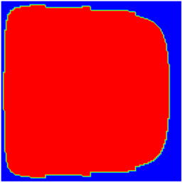 | 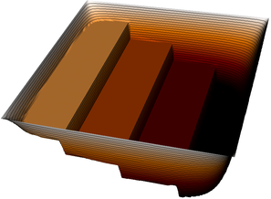 |
| 3 | 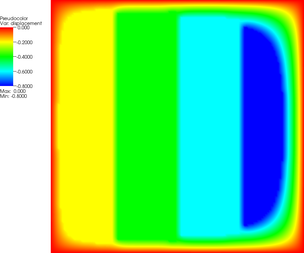 | 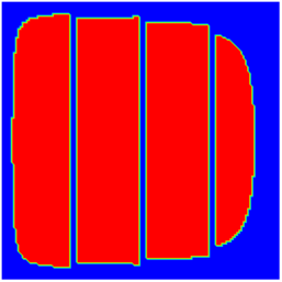 | 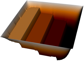 |
| 6 | 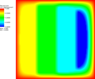 | 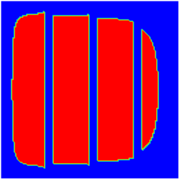 | 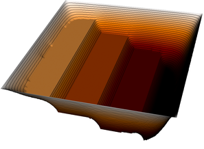 |
| 9 | 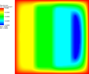 | 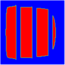 | 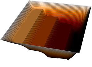 |
| 12 | 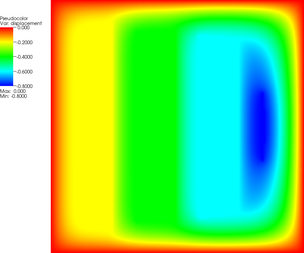 | 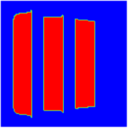 | 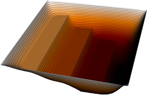 |
| 15 |  | 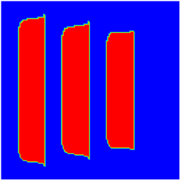 |  |
| 18 | 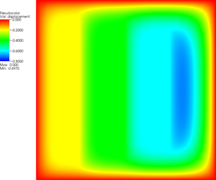 | 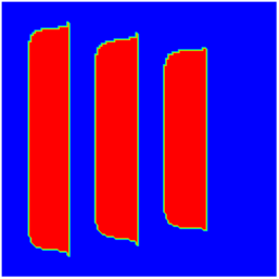 |  |
The pictures show that in the first step, the solution (which has been computed without any of the constraints active) bends through so much that pretty much every interior point has to be bounced back to the stairstep function, producing a discontinuous solution. Over the course of the active set iterations, this unphysical membrane shape is smoothed out, the contact with the lower-most stair step disappears, and the solution stabilizes.
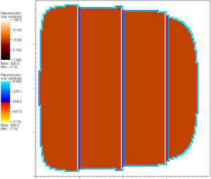
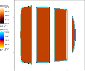
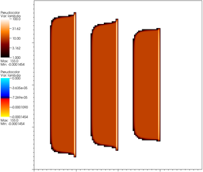
In addition to this, the program also outputs the values of the Lagrange multipliers. Remember that these are the contact forces and so should only be positive on the contact set, and zero outside. If, on the other hand, a Lagrange multiplier is negative in the active set, then this degree of freedom must be removed from the active set. The following pictures show the multipliers in iterations 1, 9 and 18, where we use red and browns to indicate positive values, and blue for negative values.
 |  |  |
| Iteration 1 | Iteration 9 | Iteration 18 |
It is easy to see that the positive values converge nicely to moderate values in the interior of the contact set and large upward forces at the edges of the steps, as one would expect (to support the large curvature of the membrane there); at the fringes of the active set, multipliers are initially negative, causing the set to shrink until, in iteration 18, there are no more negative multipliers and the algorithm has converged.
As with any of the programs of this tutorial, there are a number of obvious possibilities for extensions and experiments. The first one is clear: introduce adaptivity. Contact problems are prime candidates for adaptive meshes because the solution has lines along which it is less regular (the places where contact is established between membrane and obstacle) and other areas where the solution is very smooth (or, in the present context, constant wherever it is in contact with the obstacle). Adding this to the current program should not pose too many difficulties, but it is not trivial to find a good error estimator for that purpose.
A more challenging task would be an extension to 3d. The problem here is not so much to simply make everything run in 3d. Rather, it is that when a 3d body is deformed and gets into contact with an obstacle, then the obstacle does not act as a constraining body force within the domain as is the case here. Rather, the contact force only acts on the boundary of the object. The inequality then is not in the differential equation but in fact in the (Neumann-type) boundary conditions, though this leads to a similar kind of variational inequality. Mathematically, this means that the Lagrange multiplier only lives on the surface, though it can of course be extended by zero into the domain if that is convenient. As in the current program, one does not need to form and store this Lagrange multiplier explicitly.
A further interesting problem for the 3d case is to consider contact problems with friction. In almost every mechanical process friction has a big influence. For the modelling we have to take into account tangential stresses at the contact surface. Also we have to observe that friction adds another nonlinearity to our problem.
Another nontrivial modification is to implement a more complex constitutive law like nonlinear elasticity or elasto-plastic material behavior. The difficulty here is to handle the additional nonlinearity arising through the nonlinear constitutive law.