 |
Reference documentation for deal.II version 8.5.1
|
 |
Reference documentation for deal.II version 8.5.1
|
This program was contributed by Jean-Paul Pelteret <jppelteret@gmail.com>.
It comes without any warranty or support by its authors or the authors of deal.II.
This program is part of the deal.II code gallery and consists of the following files (click to inspect):
| 
| 
|
The Cook membrane (or cantilever) problem is a classic benchmark test for finite element formulations for solid mechanics. It is typically used to test for and demonstrate the shear-locking (or locking-free) behaviour of a finite element ansatz under quasi-incompressible conditions. As it is so widely referred to in the literature on finite-strain elasticity, we reproduce the example here. However, we consider on the compressible case to avoid many of the complexities that arise in @ref step_44 "step-44", which provides an efficient approach to deal with the quasi-incompressible case.
In this work we take a classical approach to solving the equations governing quasi-static finite-strain compressible elasticity, with code based on @ref step_44 "step-44". The formulation adopted here is that seen in many texts on solid mechanics and can be used as the starting point for extension into many topics such as material anisotropy, rate dependence or plasticity, or even as a component of multi-physics problems.
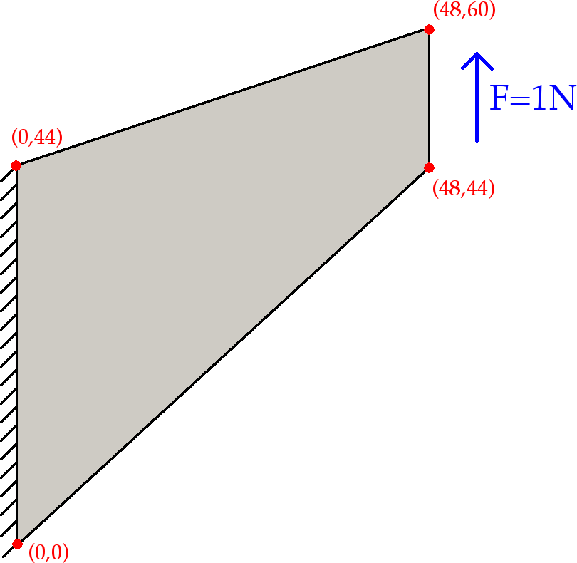
The basic problem configuration is summarised in the following image. A beam of specific dimensions is fixed at one end and a uniform traction load is applied at the other end such that the total force acting on this surface totals 1 Newton. Displacement in the third coordinate direction (out of plane) is prevented in order to impose plane strain conditions.

Note that we perform a three-dimensional computation as, for this particular formulation, the two-dimensional case corresponds to neither plane-strain nor plane-stress conditions.
Version 8.2.1 or greater of deal.II
Similar to the example programs, run
in this directory to configure the problem.
You can switch between debug and release mode by calling either
or
The problem may then be run with
If you use this program as a basis for your own work, please consider citing it in your list of references. The initial version of this work was contributed to the deal.II project by the authors listed in the following citation: J-P. V. Pelteret and A. McBride, The deal.II code gallery: Quasi-Static Finite-Strain Compressible Elasticity, 2016. DOI: 10.5281/zenodo.437601
The support of this work by the European Research Council (ERC) through the Advanced Grant 289049 MOCOPOLY is gratefully acknowledged by the first author.
C. Miehe (1994), Aspects of the formulation and finite element implementation of large strain isotropic elasticity International Journal for Numerical Methods in Engineering 37 , 12, 1981-2004. DOI: 10.1002/nme.1620371202; G.A. Holzapfel (2001), Nonlinear Solid Mechanics. A Continuum Approach for Engineering, John Wiley & Sons. ISBN: 978-0-471-82319-3; P. Wriggers (2008), Nonlinear finite element methods, Springer. DOI: 10.1007/978-3-540-71001-1; T.J.R. Hughes (2000), The Finite Element Method: Linear Static and Dynamic Finite Element Analysis, Dover. ISBN: 978-0486411811
The derivation of the finite-element problem, namely the definition and linearisation of the residual and their subsequent discretisation are quite lengthy and involved. Thankfully, the classical approach adopted in this work is well documented and therefore does not need to be reproduced here. We refer the reader to, among many other possible texts, Holzapfel (2001) and Wriggers (2008) for a detailed description of the approach applied in this work. It amounts to a reduction and slight reworking of @ref step_44 "step-44" (accounting for the removal of the two additional fields used therein). We also refer the reader to @ref step_44 "step-44" for a brief overview of the continuum mechanics and kinematics related to solid mechanics.
These results were produced using the following material properties: Shear modulus is 422.5kPa Poisson ratio is 0.3
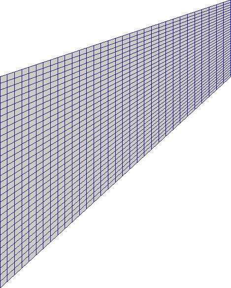
The 32x32x1 discretised reference geometry looks as follows:

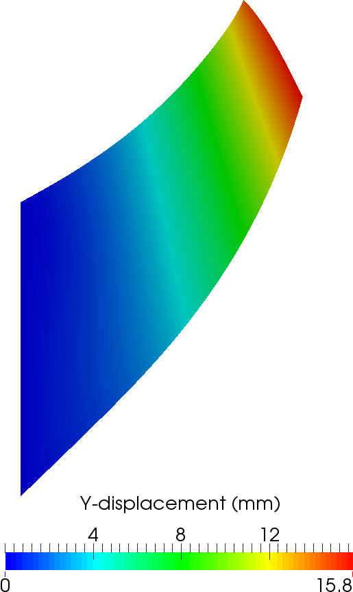
And an example of the displaced solution is given in the next image.

Below we briefly document the tip displacement as predicted for different discretisation levels and ansatz for the displacement field. A direct and, by visual inspection, favourable comparison of the following results can be made with those found in Miehe (1994). Since the material is compressible, shear-locking is not exhibited by the beam for low-order elements.
| Elements per edge | Q1 | Q2 :-— |
|---|---|---|
| 1 | 24 | 81 |
| 2 | 54 | 225 |
| 4 | 150 | 729 |
| 8 | 486 | 2601 |
| 16 | 1734 | 9801 |
| 32 | 6534 | 38025 |
| 64 | 25350 | 149769 |
| Elements per edge | Q1 | Q2 :-— |
|---|---|---|
| 1 | 5.15 | 12.19 |
| 2 | 8.72 | 13.83 |
| 4 | 12.02 | 14.22 |
| 8 | 13.61 | 14.30 |
| 16 | 14.13 | 14.32 |
| 32 | 14.28 | 14.33 |
| 64 | 14.32 | 14.33 |
We start by including all the necessary deal.II header files and some C++ related ones. They have been discussed in detail in previous tutorial programs, so you need only refer to past tutorials for details.
We then stick everything that relates to this tutorial program into a namespace of its own, and import all the deal.II function and class names into it:
There are several parameters that can be set in the code so we set up a ParameterHandler object to read in the choices at run-time.
Here we specify the polynomial order used to approximate the solution.
The quadrature order should be adjusted accordingly.
Make adjustments to the problem geometry and its discretisation.
We also need the shear modulus \mu and Poisson ration \nu for the neo-Hookean material.
Next, we choose both solver and preconditioner settings. The use of an effective preconditioner is critical to ensure convergence when a large nonlinear motion occurs within a Newton increment.
A Newton-Raphson scheme is used to solve the nonlinear system of governing equations. We now define the tolerances and the maximum number of iterations for the Newton-Raphson nonlinear solver.
Set the timestep size \varDelta t and the simulation end-time.
Finally we consolidate all of the above structures into a single container that holds all of our run-time selections.
Now we define some frequently used second and fourth-order tensors:
\mathbf{I}
\mathbf{I} \otimes \mathbf{I}
\mathcal{S}, note that as we only use this fourth-order unit tensor to operate on symmetric second-order tensors. To maintain notation consistent with Holzapfel (2001) we name the tensor \mathcal{I}
Fourth-order deviatoric tensor such that \textrm{dev} \{ \bullet \} = \{ \bullet \} - [1/\textrm{dim}][ \{ \bullet\} :\mathbf{I}]\mathbf{I}
A simple class to store time data. Its functioning is transparent so no discussion is necessary. For simplicity we assume a constant time step size.
As discussed in the literature and step-44, Neo-Hookean materials are a type of hyperelastic materials. The entire domain is assumed to be composed of a compressible neo-Hookean material. This class defines the behaviour of this material within a one-field formulation. Compressible neo-Hookean materials can be described by a strain-energy function (SEF) \Psi = \Psi_{\text{iso}}(\overline{\mathbf{b}}) + \Psi_{\text{vol}}(J) .
The isochoric response is given by \Psi_{\text{iso}}(\overline{\mathbf{b}}) = c_{1} [\overline{I}_{1} - 3] where c_{1} = \frac{\mu}{2} and \overline{I}_{1} is the first invariant of the left- or right-isochoric Cauchy-Green deformation tensors. That is \overline{I}_1 :=\textrm{tr}(\overline{\mathbf{b}}). In this example the SEF that governs the volumetric response is defined as \Psi_{\text{vol}}(J) = \kappa \frac{1}{4} [ J^2 - 1 - 2\textrm{ln}\; J ], where \kappa:= \lambda + 2/3 \mu is the bulk modulus and \lambda is Lame's first parameter.
The following class will be used to characterize the material we work with, and provides a central point that one would need to modify if one were to implement a different material model. For it to work, we will store one object of this type per quadrature point, and in each of these objects store the current state (characterized by the values or measures of the displacement field) so that we can compute the elastic coefficients linearized around the current state.
We update the material model with various deformation dependent data based on the deformation gradient \mathbf{F} and the volumetric Jacobian J = \text{det} \mathbf{F}, and at the end of the function include a physical check for internal consistency:
The second function determines the Kirchhoff stress \boldsymbol{\tau} = \boldsymbol{\tau}_{\textrm{iso}} + \boldsymbol{\tau}_{\textrm{vol}}
See Holzapfel p231 eq6.98 onwards
The fourth-order elasticity tensor in the spatial setting \mathfrak{c} is calculated from the SEF \Psi as J \mathfrak{c}_{ijkl} = F_{iA} F_{jB} \mathfrak{C}_{ABCD} F_{kC} F_{lD} where \mathfrak{C} = 4 \frac{\partial^2 \Psi(\mathbf{C})}{\partial \mathbf{C} \partial \mathbf{C}}
Derivative of the volumetric free energy with respect to J return \frac{\partial \Psi_{\text{vol}}(J)}{\partial J}
Second derivative of the volumetric free energy wrt J. We need the following computation explicitly in the tangent so we make it public. We calculate \frac{\partial^2 \Psi_{\textrm{vol}}(J)}{\partial J \partial J}
The next few functions return various data that we choose to store with the material:
Define constitutive model parameters \kappa (bulk modulus) and the neo-Hookean model parameter c_1:
Model specific data that is convenient to store with the material:
The following functions are used internally in determining the result of some of the public functions above. The first one determines the volumetric Kirchhoff stress \boldsymbol{\tau}_{\textrm{vol}}. Note the difference in its definition when compared to step-44.
Next, determine the isochoric Kirchhoff stress \boldsymbol{\tau}_{\textrm{iso}} = \mathcal{P}:\overline{\boldsymbol{\tau}}:
Then, determine the fictitious Kirchhoff stress \overline{\boldsymbol{\tau}}:
Calculate the volumetric part of the tangent J \mathfrak{c}_\textrm{vol}. Again, note the difference in its definition when compared to step-44. The extra terms result from two quantities in \boldsymbol{\tau}_{\textrm{vol}} being dependent on \boldsymbol{F}.
See Holzapfel p265
Calculate the isochoric part of the tangent J \mathfrak{c}_\textrm{iso}:
Calculate the fictitious elasticity tensor \overline{\mathfrak{c}}. For the material model chosen this is simply zero:
As seen in step-18, the PointHistory class offers a method for storing data at the quadrature points. Here each quadrature point holds a pointer to a material description. Thus, different material models can be used in different regions of the domain. Among other data, we choose to store the Kirchhoff stress \boldsymbol{\tau} and the tangent J\mathfrak{c} for the quadrature points.
The first function is used to create a material object and to initialize all tensors correctly: The second one updates the stored values and stresses based on the current deformation measure \textrm{Grad}\mathbf{u}_{\textrm{n}}.
To this end, we calculate the deformation gradient \mathbf{F} from the displacement gradient \textrm{Grad}\ \mathbf{u}, i.e. \mathbf{F}(\mathbf{u}) = \mathbf{I} + \textrm{Grad}\ \mathbf{u} and then let the material model associated with this quadrature point update itself. When computing the deformation gradient, we have to take care with which data types we compare the sum \mathbf{I} + \textrm{Grad}\ \mathbf{u}: Since I has data type SymmetricTensor, just writing I + Grad_u_n would convert the second argument to a symmetric tensor, perform the sum, and then cast the result to a Tensor (i.e., the type of a possibly nonsymmetric tensor). However, since Grad_u_n is nonsymmetric in general, the conversion to SymmetricTensor will fail. We can avoid this back and forth by converting I to Tensor first, and then performing the addition as between nonsymmetric tensors:
The material has been updated so we now calculate the Kirchhoff stress \mathbf{\tau}, the tangent J\mathfrak{c} and the first and second derivatives of the volumetric free energy.
We also store the inverse of the deformation gradient since we frequently use it:
We offer an interface to retrieve certain data. Here are the kinematic variables:
...and the kinetic variables. These are used in the material and global tangent matrix and residual assembly operations:
And finally the tangent:
In terms of member functions, this class stores for the quadrature point it represents a copy of a material type in case different materials are used in different regions of the domain, as well as the inverse of the deformation gradient...
... and stress-type variables along with the tangent J\mathfrak{c}:
The Solid class is the central class in that it represents the problem at hand. It follows the usual scheme in that all it really has is a constructor, destructor and a run() function that dispatches all the work to private functions of this class:
In the private section of this class, we first forward declare a number of objects that are used in parallelizing work using the WorkStream object (see the Parallel computing with multiple processors accessing shared memory module for more information on this).
We declare such structures for the computation of tangent (stiffness) matrix, right hand side, and for updating quadrature points:
We start the collection of member functions with one that builds the grid:
Set up the finite element system to be solved:
Several functions to assemble the system and right hand side matrices using multithreading. Each of them comes as a wrapper function, one that is executed to do the work in the WorkStream model on one cell, and one that copies the work done on this one cell into the global object that represents it:
Apply Dirichlet boundary conditions on the displacement field
Create and update the quadrature points. Here, no data needs to be copied into a global object, so the copy_local_to_global function is empty:
Solve for the displacement using a Newton-Raphson method. We break this function into the nonlinear loop and the function that solves the linearized Newton-Raphson step:
Solution retrieval as well as post-processing and writing data to file :
Finally, some member variables that describe the current state: A collection of the parameters used to describe the problem setup...
...the volume of the reference and current configurations...
...and description of the geometry on which the problem is solved:
Also, keep track of the current time and the time spent evaluating certain functions
A storage object for quadrature point information. See step-18 for more on this:
A description of the finite-element system including the displacement polynomial degree, the degree-of-freedom handler, number of DoFs per cell and the extractor objects used to retrieve information from the solution vectors:
Description of how the block-system is arranged. There is just 1 block, that contains a vector DOF \mathbf{u}. There are two reasons that we retain the block system in this problem. The first is pure laziness to perform further modifications to the code from which this work originated. The second is that a block system would typically necessary when extending this code to multiphysics problems.
Rules for Gauss-quadrature on both the cell and faces. The number of quadrature points on both cells and faces is recorded.
Objects that store the converged solution and right-hand side vectors, as well as the tangent matrix. There is a ConstraintMatrix object used to keep track of constraints. We make use of a sparsity pattern designed for a block system.
Then define a number of variables to store norms and update norms and normalisation factors.
Methods to calculate error measures
Print information to screen in a pleasing way...
Solid classWe initialise the Solid class using data extracted from the parameter file.
The Finite Element System is composed of dim continuous displacement DOFs.
The class destructor simply clears the data held by the DOFHandler
In solving the quasi-static problem, the time becomes a loading parameter, i.e. we increasing the loading linearly with time, making the two concepts interchangeable. We choose to increment time linearly using a constant time step size.
We start the function with preprocessing, and then output the initial grid before starting the simulation proper with the first time (and loading) increment.
We then declare the incremental solution update \varDelta \mathbf{\Xi}:= \{\varDelta \mathbf{u}\} and start the loop over the time domain.
At the beginning, we reset the solution update for this time step...
...solve the current time step and update total solution vector \mathbf{\Xi}_{\textrm{n}} = \mathbf{\Xi}_{\textrm{n-1}} + \varDelta \mathbf{\Xi}...
...and plot the results before moving on happily to the next time step:
Lastly, we print the vertical tip displacement of the Cook cantilever after the full load is applied
The first group of private member functions is related to parallization. We use the Threading Building Blocks library (TBB) to perform as many computationally intensive distributed tasks as possible. In particular, we assemble the tangent matrix and right hand side vector, and update data stored at the quadrature points using TBB. Our main tool for this is the WorkStream class (see the Parallel computing with multiple processors accessing shared memory module for more information).
Firstly we deal with the tangent matrix assembly structures. The PerTaskData object stores local contributions.
On the other hand, the ScratchData object stores the larger objects such as the shape-function values array (Nx) and a shape function gradient and symmetric gradient vector which we will use during the assembly.
Next, the same approach is used for the right-hand side assembly. The PerTaskData object again stores local contributions and the ScratchData object the shape function object and precomputed values vector:
And finally we define the structures to assist with updating the quadrature point information. We do not need the PerTaskData object (since there is nothing to store here) but must define one nonetheless. Note that this is because for the operation that we have here – updating the data on quadrature points – the operation is purely local: the things we do on every cell get consumed on every cell, without any global aggregation operation as is usually the case when using the WorkStream class. The fact that we still have to define a per-task data structure points to the fact that the WorkStream class may be ill-suited to this operation (we could, in principle simply create a new task using Threads::new_task for each cell) but there is not much harm done to doing it this way anyway. Furthermore, should there be different material models associated with a quadrature point, requiring varying levels of computational expense, then the method used here could be advantageous.
The ScratchData object will be used to store an alias for the solution vector so that we don't have to copy this large data structure. We then define a number of vectors to extract the solution values and gradients at the quadrature points.
On to the first of the private member functions. Here we create the triangulation of the domain, for which we choose a scaled an anisotripically discretised rectangle which is subsequently transformed into the correct of the Cook cantilever. Each relevant boundary face is then given a boundary ID number.
We then determine the volume of the reference configuration and print it for comparison.
Divide the beam, but only along the x- and y-coordinate directions
Only allow one element through the thickness (modelling a plane strain condition)
Since we wish to apply a Neumann BC to the right-hand surface, we must find the cell faces in this part of the domain and mark them with a distinct boundary ID number. The faces we are looking for are on the +x surface and will get boundary ID 11. Dirichlet boundaries exist on the left-hand face of the beam (this fixed boundary will get ID 1) and on the +Z and -Z faces (which correspond to ID 2 and we will use to impose the plane strain condition)
Transform the hyper-rectangle into the beam shape
Next we describe how the FE system is setup. We first determine the number of components per block. Since the displacement is a vector component, the first dim components belong to it.
The DOF handler is then initialised and we renumber the grid in an efficient manner. We also record the number of DOFs per block.
Setup the sparsity pattern and tangent matrix
Naturally, for a one-field vector-valued problem, all of the components of the system are coupled.
We then set up storage vectors
...and finally set up the quadrature point history:
The method used to store quadrature information is already described in step-18 and step-44. Here we implement a similar setup for a SMP machine.
Firstly the actual QPH data objects are created. This must be done only once the grid is refined to its finest level.
Next we setup the initial quadrature point data:
As the update of QP information occurs frequently and involves a number of expensive operations, we define a multithreaded approach to distributing the task across a number of CPU cores.
To start this, we first we need to obtain the total solution as it stands at this Newton increment and then create the initial copy of the scratch and copy data objects:
We then pass them and the one-cell update function to the WorkStream to be processed:
Now we describe how we extract data from the solution vector and pass it along to each QP storage object for processing.
We first need to find the solution gradients at quadrature points inside the current cell and then we update each local QP using the displacement gradient:
The next function is the driver method for the Newton-Raphson scheme. At its top we create a new vector to store the current Newton update step, reset the error storage objects and print solver header.
We now perform a number of Newton iterations to iteratively solve the nonlinear problem. Since the problem is fully nonlinear and we are using a full Newton method, the data stored in the tangent matrix and right-hand side vector is not reusable and must be cleared at each Newton step. We then initially build the right-hand side vector to check for convergence (and store this value in the first iteration). The unconstrained DOFs of the rhs vector hold the out-of-balance forces. The building is done before assembling the system matrix as the latter is an expensive operation and we can potentially avoid an extra assembly process by not assembling the tangent matrix when convergence is attained.
We can now determine the normalised residual error and check for solution convergence:
If we have decided that we want to continue with the iteration, we assemble the tangent, make and impose the Dirichlet constraints, and do the solve of the linearized system:
We can now determine the normalised Newton update error, and perform the actual update of the solution increment for the current time step, update all quadrature point information pertaining to this new displacement and stress state and continue iterating:
At the end, if it turns out that we have in fact done more iterations than the parameter file allowed, we raise an exception that can be caught in the main() function. The call AssertThrow(condition, exc_object) is in essence equivalent to if (!cond) throw exc_object; but the former form fills certain fields in the exception object that identify the location (filename and line number) where the exception was raised to make it simpler to identify where the problem happened.
This program prints out data in a nice table that is updated on a per-iteration basis. The next two functions set up the table header and footer:
At the end we also output the result that can be compared to that found in the literature, namely the displacement at the upper right corner of the beam.
if (cell->point_inside(soln_pt) == true)
Extract y-component of solution at the given point This point is coindicent with a vertex, so we can extract it directly as we're using FE_Q finite elements that have support at the vertices
Sanity check using alternate method to extract the solution at the given point. To do this, we must create an FEValues instance to help us extract the solution value at the desired point
Extract y-component of solution at given point
Determine the true residual error for the problem. That is, determine the error in the residual for the unconstrained degrees of freedom. Note that to do so, we need to ignore constrained DOFs by setting the residual in these vector components to zero.
Determine the true Newton update error for the problem
This function provides the total solution, which is valid at any Newton step. This is required as, to reduce computational error, the total solution is only updated at the end of the timestep.
Since we use TBB for assembly, we simply setup a copy of the data structures required for the process and pass them, along with the memory addresses of the assembly functions to the WorkStream object for processing. Note that we must ensure that the matrix is reset before any assembly operations can occur.
This function adds the local contribution to the system matrix. Note that we choose not to use the constraint matrix to do the job for us because the tangent matrix and residual processes have been split up into two separate functions.
Of course, we still have to define how we assemble the tangent matrix contribution for a single cell. We first need to reset and initialise some of the scratch data structures and retrieve some basic information regarding the DOF numbering on this cell. We can precalculate the cell shape function gradients. Note that the shape function gradients are defined with regard to the current configuration. That is \textrm{grad}\ \boldsymbol{\varphi} = \textrm{Grad}\ \boldsymbol{\varphi} \ \mathbf{F}^{-1}.
Now we build the local cell stiffness matrix. Since the global and local system matrices are symmetric, we can exploit this property by building only the lower half of the local matrix and copying the values to the upper half.
In doing so, we first extract some configuration dependent variables from our QPH history objects for the current quadrature point.
Next we define some aliases to make the assembly process easier to follow
This is the \mathsf{\mathbf{k}}_{\mathbf{u} \mathbf{u}} contribution. It comprises a material contribution, and a geometrical stress contribution which is only added along the local matrix diagonals:
Finally, we need to copy the lower half of the local matrix into the upper half:
The assembly of the right-hand side process is similar to the tangent matrix, so we will not describe it in too much detail. Note that since we are describing a problem with Neumann BCs, we will need the face normals and so must specify this in the update flags.
We first compute the contributions from the internal forces. Note, by definition of the rhs as the negative of the residual, these contributions are subtracted.
Next we assemble the Neumann contribution. We first check to see it the cell face exists on a boundary on which a traction is applied and add the contribution if this is the case.
We specify the traction in reference configuration. For this problem, a defined total vertical force is applied in the reference configuration. The direction of the applied traction is assumed not to evolve with the deformation of the domain.
Note that the contributions to the right hand side vector we compute here only exist in the displacement components of the vector.
The constraints for this problem are simple to describe. However, since we are dealing with an iterative Newton method, it should be noted that any displacement constraints should only be specified at the zeroth iteration and subsequently no additional contributions are to be made since the constraints are already exactly satisfied.
Since the constraints are different at different Newton iterations, we need to clear the constraints matrix and completely rebuild it. However, after the first iteration, the constraints remain the same and we can simply skip the rebuilding step if we do not clear it.
The boundary conditions for the indentation problem are as follows: On the -x, -y and -z faces (ID's 0,2,4) we set up a symmetry condition to allow only planar movement while the +x and +y faces (ID's 1,3) are traction free. In this contrived problem, part of the +z face (ID 5) is set to have no motion in the x- and y-component. Finally, as described earlier, the other part of the +z face has an the applied pressure but is also constrained in the x- and y-directions.
In the following, we will have to tell the function interpolation boundary values which components of the solution vector should be constrained (i.e., whether it's the x-, y-, z-displacements or combinations thereof). This is done using ComponentMask objects (see GlossComponentMask) which we can get from the finite element if we provide it with an extractor object for the component we wish to select. To this end we first set up such extractor objects and later use it when generating the relevant component masks:
Fixed left hand side of the beam
Zero Z-displacement through thickness direction This corresponds to a plane strain condition being imposed on the beam
As the system is composed of a single block, defining a solution scheme for the linear problem is straight-forward.
We solve for the incremental displacement d\mathbf{u}.
We've chosen by default a SSOR preconditioner as it appears to provide the fastest solver convergence characteristics for this problem on a single-thread machine. However, for multicore computing, the Jacobi preconditioner which is multithreaded may converge quicker for larger linear systems.
Otherwise if the problem is small enough, a direct solver can be utilised.
Now that we have the displacement update, distribute the constraints back to the Newton update:
Here we present how the results are written to file to be viewed using ParaView or Visit. The method is similar to that shown in the tutorials so will not be discussed in detail.
Since we are dealing with a large deformation problem, it would be nice to display the result on a displaced grid! The MappingQEulerian class linked with the DataOut class provides an interface through which this can be achieved without physically moving the grid points in the Triangulation object ourselves. We first need to copy the solution to a temporary vector and then create the Eulerian mapping. We also specify the polynomial degree to the DataOut object in order to produce a more refined output data set when higher order polynomials are used.
Lastly we provide the main driver function which appears no different to the other tutorials.
 1.8.14