 |
Reference documentation for deal.II version 9.6.0
|
 |
Reference documentation for deal.II version 9.6.0
|
This tutorial depends on step-23.
| Table of contents | |
|---|---|
This program grew out of a student project by Xing Jin at Texas A&M University. Most of the work for this program is by her. Some of the work on this tutorial program has been funded by NSF under grant DMS-0604778.
The program is part of a project that aims to simulate thermoacoustic tomography imaging. In thermoacoustic tomography, pulsed electromagnetic energy is delivered into biological issues. Tissues absorb some of this energy and those parts of the tissue that absorb the most energy generate thermoacoustic waves through thermoelastic expansion. For imaging, one uses that different kinds of tissue, most importantly healthy and diseased tissue, absorb different amounts of energy and therefore expand at different rates. The experimental setup is to measure the amplitude of the pressure waves generated by these sources on the surface of the tissue and try to reconstruct the source distributions, which is indicative for the distribution of absorbers and therefore of different kinds of tissue. Part of this project is to compare simulated data with actual measurements, so one has to solve the "forward problem", i.e. the wave equation that describes the propagation of pressure waves in tissue. This program is therefore a continuation of step-23, where the wave equation was first introduced.
The temperature at a given location, neglecting thermal diffusion, can be stated as
\rho C_p \frac{\partial}{\partial t}T(t,\mathbf r) = H(t,\mathbf r)
Here \rho (\mathbf r) is the density; C_p (\mathbf r) is the specific heat; \frac{\partial T}{\partial t}(t,\mathbf r) is the temperature rise due to the delivered microwave energy; and H(t,\mathbf r) is the heating function defined as the thermal energy per time and volume transformed from deposited microwave energy.
Let us assume that tissues have heterogeneous dielectric properties but homogeneous acoustic properties. The basic acoustic generation equation in an acoustically homogeneous medium can be described as follows: if u is the vector-valued displacement, then tissue certainly reacts to changes in pressure by acceleration:
\rho \frac{\partial^2}{\partial t^2}u(t,\mathbf r) = -\nabla p(t,\mathbf r).
Furthermore, it contracts due to excess pressure and expands based on changes in temperature:
\nabla \cdot u(t,\mathbf r) = -\frac{p(t,\mathbf r)}{\rho c_0^2}+\beta T(t,\mathbf r) .
Here, \beta is a thermoexpansion coefficient.
Let us now make the assumption that heating only happens on a time scale much shorter than wave propagation through tissue (i.e. the temporal length of the microwave pulse that heats the tissue is much shorter than the time it takes a wave to cross the domain). In that case, the heating rate H(t,\mathbf r) can be written as H(t,\mathbf r) = a(\mathbf r)\delta(t) (where a(\mathbf r) is a map of absorption strengths for microwave energy and \delta(t) is the Dirac delta function), which together with the first equation above will yield an instantaneous jump in the temperature T(\mathbf r) at time t=0. Using this assumption, and taking all equations together, we can rewrite and combine the above as follows:
\Delta p-\frac{1}{c_0^2} \frac{\partial^2 p}{\partial t^2} = \lambda a(\mathbf r)\frac{d\delta(t)}{dt}
where \lambda = - \frac{\beta}{C_p}.
This somewhat strange equation with the derivative of a Dirac delta function on the right hand side can be rewritten as an initial value problem as follows:
\begin{eqnarray*} \Delta \bar{p}- \frac{1}{c_0^2} \frac{\partial^2 \bar{p}}{\partial t^2} & = & 0 \\ \bar{p}(0,\mathbf r) &=& c_0^2 \lambda a(\mathbf r) = b(\mathbf r) \\ \frac{\partial\bar{p}(0,\mathbf r)}{\partial t} &=& 0. \end{eqnarray*}
(A derivation of this transformation into an initial value problem is given at the end of this introduction as an appendix.)
In the inverse problem, it is the initial condition b(\mathbf r) = c_0^2 \lambda a(\mathbf r) that one would like to recover, since it is a map of absorption strengths for microwave energy, and therefore presumably an indicator to discern healthy from diseased tissue.
In real application, the thermoacoustic source is very small as compared to the medium. The propagation path of the thermoacoustic waves can then be approximated as from the source to the infinity. Furthermore, detectors are only a limited distance from the source. One only needs to evaluate the values when the thermoacoustic waves pass through the detectors, although they do continue beyond. This is therefore a problem where we are only interested in a small part of an infinite medium, and we do not want waves generated somewhere to be reflected at the boundary of the domain which we consider interesting. Rather, we would like to simulate only that part of the wave field that is contained inside the domain of interest, and waves that hit the boundary of that domain to simply pass undisturbed through the boundary. In other words, we would like the boundary to absorb any waves that hit it.
In general, this is a hard problem: Good absorbing boundary conditions are nonlinear and/or numerically very expensive. We therefore opt for a simple first order approximation to absorbing boundary conditions that reads
\frac{\partial\bar{p}}{\partial\mathbf n} = -\frac{1}{c_0} \frac{\partial\bar{p}}{\partial t}
Here, \frac{\partial\bar{p}}{\partial\mathbf n} is the normal derivative at the boundary. It should be noted that this is not a particularly good boundary condition, but it is one of the very few that are reasonably simple to implement.
As in step-23, one first introduces a second variable, which is defined as the derivative of the pressure potential:
v = \frac{\partial\bar{p}}{\partial t}
With the second variable, one then transforms the forward problem into two separate equations:
\begin{eqnarray*} \bar{p}_{t} - v & = & 0 \\ \Delta\bar{p} - \frac{1}{c_0^2}\,v_{t} & = & f \end{eqnarray*}
with initial conditions:
\begin{eqnarray*} \bar{p}(0,\mathbf r) & = & b(r) \\ v(0,\mathbf r)=\bar{p}_t(0,\mathbf r) & = & 0. \end{eqnarray*}
Note that we have introduced a right hand side f(t,\mathbf r) here to show how to derive these formulas in the general case, although in the application to the thermoacoustic problem f=0.
The semi-discretized, weak version of this model, using the general \theta scheme introduced in step-23 is then:
\begin{eqnarray*} \left(\frac{\bar{p}^n-\bar{p}^{n-1}}{k},\phi\right)_\Omega- \left(\theta v^{n}+(1-\theta)v^{n-1},\phi\right)_\Omega & = & 0 \\ -\left(\nabla((\theta\bar{p}^n+(1-\theta)\bar{p}^{n-1})),\nabla\phi\right)_\Omega- \frac{1}{c_0}\left(\frac{\bar{p}^n-\bar{p}^{n-1}}{k},\phi\right)_{\partial\Omega} - \frac{1}{c_0^2}\left(\frac{v^n-v^{n-1}}{k},\phi\right)_\Omega & = & \left(\theta f^{n}+(1-\theta)f^{n-1}, \phi\right)_\Omega, \end{eqnarray*}
where \phi is an arbitrary test function, and where we have used the absorbing boundary condition to integrate by parts: absorbing boundary conditions are incorporated into the weak form by using
\int_\Omega\varphi \, \Delta p\; dx = -\int_\Omega\nabla \varphi \cdot \nabla p dx + \int_{\partial\Omega}\varphi \frac{\partial p}{\partial {\mathbf n}}ds.
From this we obtain the discrete model by introducing a finite number of shape functions, and get
\begin{eqnarray*} M\bar{p}^{n}-k \theta M v^n & = & M\bar{p}^{n-1}+k (1-\theta)Mv^{n-1},\\ (-c_0^2k \theta A-c_0 B)\bar{p}^n-Mv^{n} & = & (c_0^2k(1-\theta)A-c_0B)\bar{p}^{n-1}-Mv^{n-1}+c_0^2k(\theta F^{n}+(1-\theta)F^{n-1}). \end{eqnarray*}
The matrices M and A are here as in step-23, and the boundary mass matrix
B_{ij} = \left(\varphi_i,\varphi_j\right)_{\partial\Omega}
results from the use of absorbing boundary conditions.
Above two equations can be rewritten in a matrix form with the pressure and its derivative as an unknown vector:
\left(\begin{array}{cc} M & -k\theta M \\ c_0^2\,k\,\theta\,A+c_0\,B & M \\ \end{array} \right)\\ \left(\begin{array}{c} \bar{p}^{n} \\ \bar{v}^{n} \end{array}\right)=\\ \left(\begin{array}{l} G_1 \\ G_2 -(\theta F^{n}+(1-\theta)F ^{n-1})c_{0}^{2}k \\ \end{array}\right)
where
\left(\begin{array}{c} G_1 \\ G_2 \\ \end{array} \right)=\\ \left(\begin{array}{l} M\bar{p}^{n-1}+k(1-\theta)Mv^{n-1}\\ (-c_{0}^{2}k (1-\theta)A+c_0 B)\bar{p}^{n-1} +Mv^{n-1} \end{array}\right)
By simple transformations, one then obtains two equations for the pressure potential and its derivative, just as in the previous tutorial program:
\begin{eqnarray*} (M+(k\,\theta\,c_{0})^{2}A+c_0k\theta B)\bar{p}^{n} & = & G_{1}+(k\, \theta)G_{2}-(c_0k)^2\theta (\theta F^{n}+(1-\theta)F^{n-1}) \\ Mv^n & = & -(c_0^2\,k\, \theta\, A+c_0B)\bar{p}^{n}+ G_2 - c_0^2k(\theta F^{n}+(1-\theta)F^{n-1}) \end{eqnarray*}
Compared to step-23, this programs adds the treatment of a simple absorbing boundary conditions. In addition, it deals with data obtained from actual experimental measurements. To this end, we need to evaluate the solution at points at which the experiment also evaluates a real pressure field. We will see how to do that using the VectorTools::point_value function further down below.
In the derivation of the initial value problem for the wave equation, we initially found that the equation had the derivative of a Dirac delta function as a right hand side:
\Delta p-\frac{1}{c_0^2} \frac{\partial^2 p}{\partial t^2} = \lambda a(\mathbf r)\frac{d\delta(t)}{dt}.
In order to see how to transform this single equation into the usual statement of a PDE with initial conditions, let us make the assumption that the physically quite reasonable medium is at rest initially, i.e. p(t,\mathbf r)=\frac{\partial p(t,\mathbf r)}{\partial t}=0 for t<0. Next, let us form the indefinite integral with respect to time of both sides:
\int^t \Delta p\; dt -\int^t \frac{1}{c_0^2} \frac{\partial^2 p}{\partial t^2} \; dt = \int^t \lambda a(\mathbf r)\frac{d\delta(t)}{dt} \;dt.
This immediately leads to the statement
P(t,\mathbf r) - \frac{1}{c_0^2} \frac{\partial p}{\partial t} = \lambda a(\mathbf r) \delta(t),
where P(t,\mathbf r) is such that \frac{dP(t,\mathbf r)}{dt}=\Delta p. Next, we form the (definite) integral over time from t=-\epsilon to t=+\epsilon to find
\int_{-\epsilon}^{\epsilon} P(t,\mathbf r)\; dt - \frac{1}{c_0^2} \left[ p(\epsilon,\mathbf r) - p(-\epsilon,\mathbf r) \right] = \int_{-\epsilon}^{\epsilon} \lambda a(\mathbf r) \delta(t) \; dt.
If we use the property of the delta function that \int_{-\epsilon}^{\epsilon} \delta(t)\; dt = 1, and assume that P is a continuous function in time, we find as we let \epsilon go to zero that
- \lim_{\epsilon\rightarrow 0}\frac{1}{c_0^2} \left[ p(\epsilon,\mathbf r) - p(-\epsilon,\mathbf r) \right] = \lambda a(\mathbf r).
In other words, using that p(-\epsilon,\mathbf r)=0, we retrieve the initial condition
\frac{1}{c_0^2} p(0,\mathbf r) = \lambda a(\mathbf r).
At the same time, we know that for every t>0 the delta function is zero, so for 0<t<T we get the equation
\Delta p-\frac{1}{c_0^2} \frac{\partial^2 p}{\partial t^2} = 0.
Consequently, we have obtained a representation of the wave equation and one initial condition from the original somewhat strange equation.
Finally, because we here have an equation with two time derivatives, we still need a second initial condition. To this end, let us go back to the equation
\Delta p-\frac{1}{c_0^2} \frac{\partial^2 p}{\partial t^2} = \lambda a(\mathbf r)\frac{d\delta(t)}{dt}.
and integrate it in time from t=-\epsilon to t=+\epsilon. This leads to
P(\epsilon)-P(-\epsilon) -\frac{1}{c_0^2} \left[\frac{\partial p(\epsilon)}{\partial t} - \frac{\partial p(-\epsilon)}{\partial t}\right] = \lambda a(\mathbf r) \int_{-\epsilon}^{\epsilon}\frac{d\delta(t)}{dt} \; dt.
Using integration by parts of the form
\int_{-\epsilon}^{\epsilon}\varphi(t)\frac{d\delta(t)}{dt} \; dt = -\int_{-\epsilon}^{\epsilon}\frac{d\varphi(t)}{dt} \delta(t)\; dt
where we use that \delta(\pm \epsilon)=0 and inserting \varphi(t)=1, we see that in fact
\int_{-\epsilon}^{\epsilon}\frac{d\delta(t)}{dt} \; dt = 0.
Now, let \epsilon\rightarrow 0. Assuming that P is a continuous function in time, we see that
P(\epsilon)-P(-\epsilon) \rightarrow 0,
and consequently
\frac{\partial p(\epsilon)}{\partial t} - \frac{\partial p(-\epsilon)}{\partial t} \rightarrow 0.
However, we have assumed that \frac{\partial p(-\epsilon)}{\partial t}=0. Consequently, we obtain as the second initial condition that
\frac{\partial p(0)}{\partial t} = 0,
completing the system of equations.
The following have all been covered previously:
This is the only new one: We will need a library function defined in the namespace GridTools that computes the minimal cell diameter.
The last step is as in all previous programs:
The first part of the main class is exactly as in step-23 (except for the name):
Here's what's new: first, we need that boundary mass matrix B that came out of the absorbing boundary condition. Likewise, since this time we consider a realistic medium, we must have a measure of the wave speed c_0 that will enter all the formulas with the Laplace matrix (which we still define as (\nabla \phi_i,\nabla \phi_j)):
The last thing we have to take care of is that we wanted to evaluate the solution at a certain number of detector locations. We need an array to hold these locations, declared here and filled in the constructor:
As usual, we have to define our initial values, boundary conditions, and right hand side functions. Things are a bit simpler this time: we consider a problem that is driven by initial conditions, so there is no right hand side function (though you could look up in step-23 to see how this can be done). Secondly, there are no boundary conditions: the entire boundary of the domain consists of absorbing boundary conditions. That only leaves initial conditions, and there things are simple too since for this particular application only nonzero initial conditions for the pressure are prescribed, not for the velocity (which is zero at the initial time).
So this is all we need: a class that specifies initial conditions for the pressure. In the physical setting considered in this program, these are small absorbers, which we model as a series of little circles where we assume that the pressure surplus is one, whereas no absorption and therefore no pressure surplus is everywhere else. This is how we do things (note that if we wanted to expand this program to not only compile but also to run, we would have to initialize the sources with three-dimensional source locations):
TATForwardProblem classLet's start again with the constructor. Setting the member variables is straightforward. We use the acoustic wave speed of mineral oil (in millimeters per microsecond, a common unit in experimental biomedical imaging) since this is where many of the experiments we want to compare the output with are made in. The Crank-Nicolson scheme is used again, i.e. theta is set to 0.5. The time step is later selected to satisfy k = \frac hc: here we initialize it to an invalid number.
The second task in the constructor is to initialize the array that holds the detector locations. The results of this program were compared with experiments in which the step size of the detector spacing is 2.25 degree, corresponding to 160 detector locations. The radius of the scanning circle is selected to be half way between the center and the boundary to avoid that the remaining reflections from the imperfect boundary condition spoils our numerical results.
The locations of the detectors are then calculated in clockwise order. Note that the following of course only works if we are computing in 2d, a condition that we guard with an assertion. If we later wanted to run the same program in 3d, we would have to add code here for the initialization of detector locations in 3d. Due to the assertion, there is no way we can forget to do this.
The following system is pretty much what we've already done in step-23, but with two important differences. First, we have to create a circular (or spherical) mesh around the origin, with a radius of 1. This nothing new: we've done so before in step-6 and step-10, where we also explain how the PolarManifold or SphericalManifold object places new points on concentric circles when a cell is refined, which we will use here as well.
One thing we had to make sure is that the time step satisfies the CFL condition discussed in the introduction of step-23. Back in that program, we ensured this by hand by setting a timestep that matches the mesh width, but that was error prone because if we refined the mesh once more we would also have to make sure the time step is changed. Here, we do that automatically: we ask a library function for the minimal diameter of any cell. Then we set k=\frac h{c_0}. The only problem is: what exactly is h? The point is that there is really no good theory on this question for the wave equation. It is known that for uniformly refined meshes consisting of rectangles, h is the minimal edge length. But for meshes on general quadrilaterals, the exact relationship appears to be unknown, i.e. it is unknown what properties of cells are relevant for the CFL condition. The problem is that the CFL condition follows from knowledge of the smallest eigenvalue of the Laplace matrix, and that can only be computed analytically for simply structured meshes.
The upshot of all this is that we're not quite sure what exactly we should take for h. The function GridTools::minimal_cell_diameter computes the minimal diameter of all cells. If the cells were all squares or cubes, then the minimal edge length would be the minimal diameter divided by std::sqrt(dim). We simply generalize this, without theoretical justification, to the case of non-uniform meshes.
The only other significant change is that we need to build the boundary mass matrix. We will comment on this further down below.
The second difference, as mentioned, to step-23 is that we need to build the boundary mass matrix that grew out of the absorbing boundary conditions.
A first observation would be that this matrix is much sparser than the regular mass matrix, since none of the shape functions with purely interior support contribute to this matrix. We could therefore optimize the storage pattern to this situation and build up a second sparsity pattern that only contains the nonzero entries that we need. There is a trade-off to make here: first, we would have to have a second sparsity pattern object, so that costs memory. Secondly, the matrix attached to this sparsity pattern is going to be smaller and therefore requires less memory; it would also be faster to perform matrix-vector multiplications with it. The final argument, however, is the one that tips the scale: we are not primarily interested in performing matrix-vector with the boundary matrix alone (though we need to do that for the right hand side vector once per time step), but mostly wish to add it up to the other matrices used in the first of the two equations since this is the one that is going to be multiplied with once per iteration of the CG method, i.e. significantly more often. It is now the case that the SparseMatrix::add class allows to add one matrix to another, but only if they use the same sparsity pattern (the reason being that we can't add nonzero entries to a matrix after the sparsity pattern has been created, so we simply require that the two matrices have the same sparsity pattern).
So let's go with that:
The second thing to do is to actually build the matrix. Here, we need to integrate over faces of cells, so first we need a quadrature object that works on dim-1 dimensional objects. Secondly, the FEFaceValues variant of FEValues that works on faces, as its name suggest. And finally, the other variables that are part of the assembly machinery. All of this we put between curly braces to limit the scope of these variables to where we actually need them.
The actual act of assembling the matrix is then fairly straightforward: we loop over all cells, over all faces of each of these cells, and then do something only if that particular face is at the boundary of the domain. Like this:
The following two functions, solving the linear systems for the pressure and the velocity variable, are taken pretty much verbatim (with the exception of the change of name from u to p of the primary variable) from step-23:
The same holds here: the function is from step-23.
This function that does most of the work is pretty much again like in step-23, though we make things a bit clearer by using the vectors G1 and G2 mentioned in the introduction. Compared to the overall memory consumption of the program, the introduction of a few temporary vectors isn't doing much harm.
The only changes to this function are: first, that we do not have to project initial values for the velocity v, since we know that it is zero. And second that we evaluate the solution at the detector locations computed in the constructor. This is done using the VectorTools::point_value function. These values are then written to a file that we open at the beginning of the function.
main functionWhat remains is the main function of the program. There is nothing here that hasn't been shown in several of the previous programs:
The program writes both graphical data for each time step as well as the values evaluated at each detector location to disk. We then draw them in plots. Experimental data were also collected for comparison. Currently our experiments have only been done in two dimensions by circularly scanning a single detector. The tissue sample here is a thin slice in the X-Y plane ( Z=0), and we assume that signals from other Z directions won't contribute to the data. Consequently, we only have to compare our experimental data with two dimensional simulated data.
This movie shows the thermoacoustic waves generated by a single small absorber propagating in the medium (in our simulation, we assume the medium is mineral oil, which has a acoustic speed of 1.437 \frac{mm}{\mu s}):
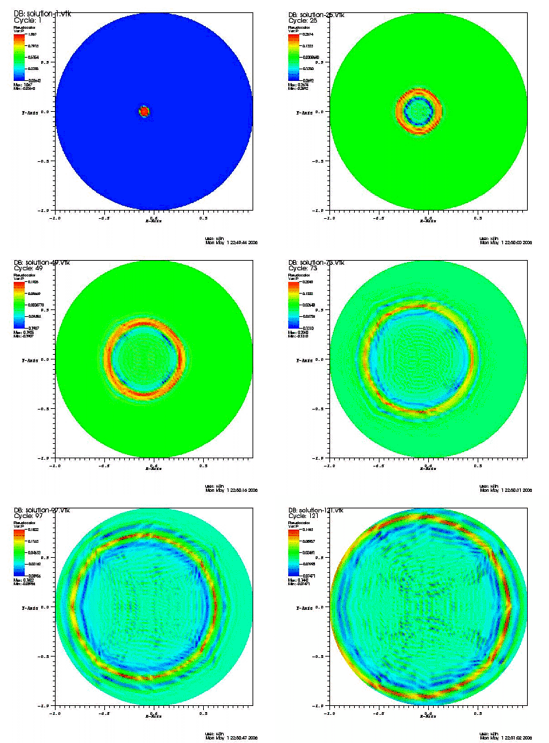
For a single absorber, we of course have to change the InitialValuesP class accordingly.
Next, let us compare experimental and computational results. The visualization uses a technique long used in seismology, where the data of each detector is plotted all in one graph. The way this is done is by offsetting each detector's signal a bit compared to the previous one. For example, here is a plot of the first four detectors (from bottom to top, with time in microseconds running from left to right) using the source setup used in the program, to make things a bit more interesting compared to the present case of only a single source:
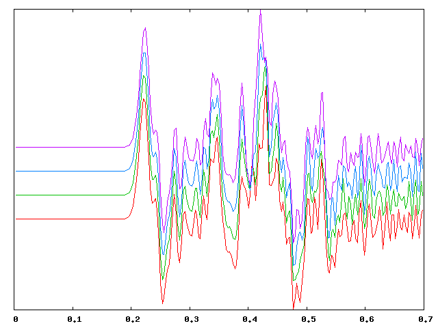
One thing that can be seen, for example, is that the arrival of the second and fourth signals shifts to earlier times for greater detector numbers (i.e. the topmost ones), but not the first and the third; this can be interpreted to mean that the origin of these signals must be closer to the latter detectors than to the former ones.
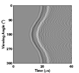
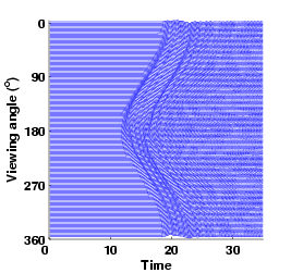
If we stack not only 4, but all 160 detectors in one graph, the individual lines blur, but where they run together they create a pattern of darker or lighter grayscales. The following two figures show the results obtained at the detector locations stacked in that way. The left figure is obtained from experiments, and the right is the simulated data. In the experiment, a single small strong absorber was embedded in weaker absorbing tissue:
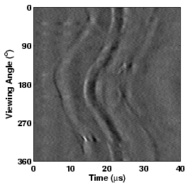 | 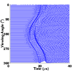 |
It is obvious that the source location is closer to the detectors at angle 180^\circ. All the other signals that can be seen in the experimental data result from the fact that there are weak absorbers also in the rest of the tissue, which surrounds the signals generated by the small strong absorber in the center. On the other hand, in the simulated data, we only simulate the small strong absorber.
In reality, detectors have limited bandwidth. The thermoacoustic waves passing through the detector will therefore be filtered. By using a high-pass filter (implemented in MATLAB and run against the data file produced by this program), the simulated results can be made to look closer to the experimental data:
In our simulations, we see spurious signals behind the main wave that result from numerical artifacts. This problem can be alleviated by using finer mesh, resulting in the following plot:
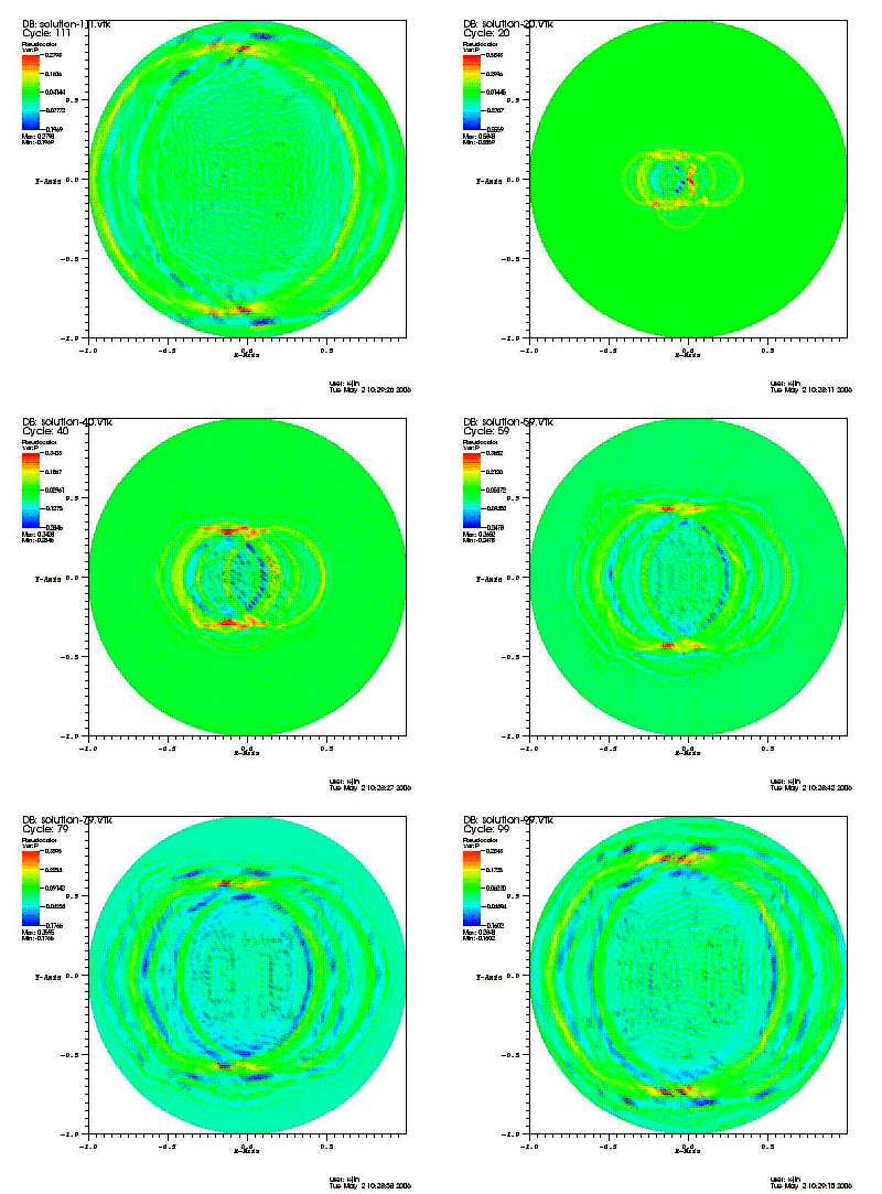
To further verify the program, we will also show simulation results for multiple absorbers. This corresponds to the case that is actually implemented in the program. The following movie shows the propagation of the generated thermoacoustic waves in the medium by multiple absorbers:
Experimental data and our simulated data are compared in the following two figures:
 | 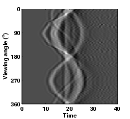 |
Note that in the experimental data, the first signal (i.e. the left-most dark line) results from absorption at the tissue boundary, and therefore reaches the detectors first and before any of the signals from the interior. This signal is also faintly visible at the end of the traces, around 30 \mu s, which indicates that the signal traveled through the entire tissue to reach detectors at the other side, after all the signals originating from the interior have reached them.
As before, the numerical result better matches experimental ones by applying a bandwidth filter that matches the actual behavior of detectors (left) and by choosing a finer mesh (right):
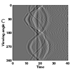 | 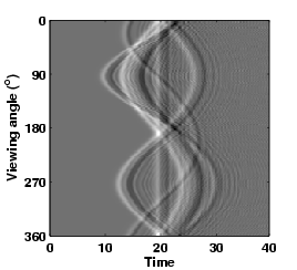 |
One of the important differences between the left and the right figure is that the curves look much less "angular" at the right. The angularity comes from the fact that while waves in the continuous equation travel equally fast in all directions, this isn't the case after discretization: there, waves that travel diagonal to cells move at slightly different speeds to those that move parallel to mesh lines. This anisotropy leads to wave fronts that aren't perfectly circular (and would produce sinusoidal signals in the stacked plots), but are bulged out in certain directions. To make things worse, the circular mesh we use (see for example step-6 for a view of the coarse mesh) is not isotropic either. The net result is that the signal fronts are not sinusoidal unless the mesh is sufficiently fine. The right image is a lot better in this respect, though artifacts in the form of trailing spurious waves can still be seen.