This tutorial depends on step-7.
Introduction
This is a variant of step-12 with the only change that we are using the MeshWorker framework with the pre-made LocalIntegrator helper classes instead of assembling the face terms using FEInterfaceValues.
The details of this framework on how it is used in practice will be explained as part of this tutorial program.
The testcase
The problem we solve here is the same as the one in step-12.
The commented program
The first few files have already been covered in previous examples and will thus not be further commented on:
#include <deal.II/base/quadrature_lib.h>
#include <deal.II/base/function.h>
#include <deal.II/lac/vector.h>
#include <deal.II/lac/dynamic_sparsity_pattern.h>
#include <deal.II/lac/sparse_matrix.h>
#include <deal.II/grid/
tria.h>
#include <deal.II/grid/grid_generator.h>
#include <deal.II/grid/grid_out.h>
#include <deal.II/grid/grid_refinement.h>
#include <deal.II/fe/fe_values.h>
#include <deal.II/fe/mapping_q1.h>
#include <deal.II/dofs/dof_handler.h>
#include <deal.II/dofs/dof_tools.h>
#include <deal.II/numerics/data_out.h>
const ::Triangulation< dim, spacedim > & tria
Here the discontinuous finite elements are defined. They are used in the same way as all other finite elements, though – as you have seen in previous tutorial programs – there isn't much user interaction with finite element classes at all: they are passed to DoFHandler and FEValues objects, and that is about it.
#include <deal.II/fe/fe_dgq.h>
We are going to use the simplest possible solver, called Richardson iteration, that represents a simple defect correction. This, in combination with a block SSOR preconditioner (defined in precondition_block.h), that uses the special block matrix structure of system matrices arising from DG discretizations.
#include <deal.II/lac/solver_richardson.h>
#include <deal.II/lac/precondition_block.h>
We are going to use gradients as refinement indicator.
#include <deal.II/numerics/derivative_approximation.h>
Here come the new include files for using the MeshWorker framework. The first contains the class MeshWorker::DoFInfo, which provides local integrators with a mapping between local and global degrees of freedom. It stores the results of local integrals as well in its base class MeshWorker::LocalResults. In the second of these files, we find an object of type MeshWorker::IntegrationInfo, which is mostly a wrapper around a group of FEValues objects. The file meshworker/simple.h contains classes assembling locally integrated data into a global system containing only a single matrix. Finally, we will need the file that runs the loop over all mesh cells and faces.
#include <deal.II/meshworker/dof_info.h>
#include <deal.II/meshworker/integration_info.h>
#include <deal.II/meshworker/simple.h>
#include <deal.II/meshworker/loop.h>
Like in all programs, we finish this section by including the needed C++ headers and declaring we want to use objects in the dealii namespace without prefix.
#include <iostream>
#include <fstream>
namespace Step12
{
Equation data
First, we define a class describing the inhomogeneous boundary data. Since only its values are used, we implement value_list(), but leave all other functions of Function undefined.
template <int dim>
class BoundaryValues :
public Function<dim>
{
public:
BoundaryValues() = default;
std::vector<double> & values,
const unsigned int component = 0) const override;
};
virtual void value_list(const std::vector< Point< dim > > &points, std::vector< RangeNumberType > &values, const unsigned int component=0) const
Given the flow direction, the inflow boundary of the unit square \([0,1]^2\) are the right and the lower boundaries. We prescribe discontinuous boundary values 1 and 0 on the x-axis and value 0 on the right boundary. The values of this function on the outflow boundaries will not be used within the DG scheme.
template <int dim>
void BoundaryValues<dim>::value_list(
const std::vector<
Point<dim>> &points,
std::vector<double> & values,
const unsigned int component) const
{
(void)component;
for (unsigned int i = 0; i < values.size(); ++i)
{
if (points[i](0) < 0.5)
values[i] = 1.;
else
values[i] = 0.;
}
}
#define AssertDimension(dim1, dim2)
#define AssertIndexRange(index, range)
Finally, a function that computes and returns the wind field \(\beta=\beta(\mathbf x)\). As explained in the introduction, we will use a rotational field around the origin in 2d. In 3d, we simply leave the \(z\)-component unset (i.e., at zero), whereas the function can not be used in 1d in its current implementation:
template <int dim>
{
Assert(dim >= 2, ExcNotImplemented());
wind_field[0] = -p[1];
wind_field[1] = p[0];
wind_field /= wind_field.
norm();
return wind_field;
}
numbers::NumberTraits< Number >::real_type norm() const
#define Assert(cond, exc)
The AdvectionProblem class
After this preparations, we proceed with the main class of this program, called AdvectionProblem. It is basically the main class of step-6. We do not have an AffineConstraints object, because there are no hanging node constraints in DG discretizations.
Major differences will only come up in the implementation of the assemble functions, since here, we not only need to cover the flux integrals over faces, we also use the MeshWorker interface to simplify the loops involved.
template <int dim>
class AdvectionProblem
{
public:
AdvectionProblem();
void run();
private:
void setup_system();
void assemble_system();
void refine_grid();
void output_results(const unsigned int cycle) const;
const ::parallel::distributed::Triangulation< dim, spacedim > * triangulation
Furthermore we want to use DG elements of degree 1 (but this is only specified in the constructor). If you want to use a DG method of a different degree the whole program stays the same, only replace 1 in the constructor by the desired polynomial degree.
The next four members represent the linear system to be solved. system_matrix and right_hand_side are generated by assemble_system(), the solution is computed in solve(). The sparsity_pattern is used to determine the location of nonzero elements in system_matrix.
Finally, we have to provide functions that assemble the cell, boundary, and inner face terms. Within the MeshWorker framework, the loop over all cells and much of the setup of operations will be done outside this class, so all we have to provide are these three operations. They will then work on intermediate objects for which first, we here define alias to the info objects handed to the local integration functions in order to make our life easier below.
The following three functions are then the ones that get called inside the generic loop over all cells and faces. They are the ones doing the actual integration.
In our code below, these functions do not access member variables of the current class, so we can mark them as static and simply pass pointers to these functions to the MeshWorker framework. If, however, these functions would want to access member variables (or needed additional arguments beyond the ones specified below), we could use the facilities of lambda functions to provide the MeshWorker framework with objects that act as if they had the required number and types of arguments, but have in fact other arguments already bound.
static void integrate_cell_term(DoFInfo &dinfo, CellInfo &info);
static void integrate_boundary_term(DoFInfo &dinfo, CellInfo &info);
static void integrate_face_term(DoFInfo & dinfo1,
DoFInfo & dinfo2,
CellInfo &info1,
CellInfo &info2);
};
We start with the constructor. The 1 in the constructor call of fe is the polynomial degree.
template <int dim>
AdvectionProblem<dim>::AdvectionProblem()
: mapping()
, fe(1)
{}
template <int dim>
void AdvectionProblem<dim>::setup_system()
{
In the function that sets up the usual finite element data structures, we first need to distribute the DoFs.
dof_handler.distribute_dofs(fe);
We start by generating the sparsity pattern. To this end, we first fill an intermediate object of type DynamicSparsityPattern with the couplings appearing in the system. After building the pattern, this object is copied to sparsity_pattern and can be discarded.
To build the sparsity pattern for DG discretizations, we can call the function analogue to DoFTools::make_sparsity_pattern, which is called DoFTools::make_flux_sparsity_pattern:
sparsity_pattern.copy_from(dsp);
void make_flux_sparsity_pattern(const DoFHandler< dim, spacedim > &dof_handler, SparsityPatternBase &sparsity_pattern)
Finally, we set up the structure of all components of the linear system.
system_matrix.reinit(sparsity_pattern);
solution.reinit(dof_handler.n_dofs());
right_hand_side.reinit(dof_handler.n_dofs());
}
The assemble_system function
Here we see the major difference to assembling by hand. Instead of writing loops over cells and faces, we leave all this to the MeshWorker framework. In order to do so, we just have to define local integration functions and use one of the classes in namespace MeshWorker::Assembler to build the global system.
template <int dim>
void AdvectionProblem<dim>::assemble_system()
{
This is the magic object, which knows everything about the data structures and local integration. This is the object doing the work in the function MeshWorker::loop(), which is implicitly called by MeshWorker::integration_loop() below. After the functions to which we provide pointers did the local integration, the MeshWorker::Assembler::SystemSimple object distributes these into the global sparse matrix and the right hand side vector.
First, we initialize the quadrature formulae and the update flags in the worker base class. For quadrature, we play safe and use a QGauss formula with number of points one higher than the polynomial degree used. Since the quadratures for cells, boundary and interior faces can be selected independently, we have to hand over this value three times.
const unsigned int n_gauss_points = dof_handler.get_fe().degree + 1;
info_box.initialize_gauss_quadrature(n_gauss_points,
n_gauss_points,
n_gauss_points);
These are the types of values we need for integrating our system. They are added to the flags used on cells, boundary and interior faces, as well as interior neighbor faces, which is forced by the four true values.
info_box.initialize_update_flags();
info_box.add_update_flags(update_flags, true, true, true, true);
@ update_values
Shape function values.
@ update_gradients
Shape function gradients.
@ update_quadrature_points
Transformed quadrature points.
After preparing all data in info_box, we initialize the FEValues objects in there.
info_box.initialize(fe, mapping);
The object created so far helps us do the local integration on each cell and face. Now, we need an object which receives the integrated (local) data and forwards them to the assembler.
Now, we have to create the assembler object and tell it, where to put the local data. These will be our system matrix and the right hand side.
assembler;
assembler.initialize(system_matrix, right_hand_side);
Finally, the integration loop over all active cells (determined by the first argument, which is an active iterator).
As noted in the discussion when declaring the local integration functions in the class declaration, the arguments expected by the assembling integrator class are not actually function pointers. Rather, they are objects that can be called like functions with a certain number of arguments. Consequently, we could also pass objects with appropriate operator() implementations here, or lambda functions if the local integrators were, for example, non-static member functions.
dim,
dof_handler.begin_active(),
dof_handler.end(),
dof_info,
info_box,
&AdvectionProblem<dim>::integrate_cell_term,
&AdvectionProblem<dim>::integrate_boundary_term,
&AdvectionProblem<dim>::integrate_face_term,
assembler);
}
void loop(ITERATOR begin, std_cxx20::type_identity_t< ITERATOR > end, DOFINFO &dinfo, INFOBOX &info, const std::function< void(DOFINFO &, typename INFOBOX::CellInfo &)> &cell_worker, const std::function< void(DOFINFO &, typename INFOBOX::CellInfo &)> &boundary_worker, const std::function< void(DOFINFO &, DOFINFO &, typename INFOBOX::CellInfo &, typename INFOBOX::CellInfo &)> &face_worker, ASSEMBLER &assembler, const LoopControl &lctrl=LoopControl())
The local integrators
These are the functions given to the MeshWorker::integration_loop() called just above. They compute the local contributions to the system matrix and right hand side on cells and faces.
template <int dim>
void AdvectionProblem<dim>::integrate_cell_term(DoFInfo & dinfo,
CellInfo &info)
{
First, let us retrieve some of the objects used here from info. Note that these objects can handle much more complex structures, thus the access here looks more complicated than might seem necessary.
const std::vector<double> &JxW = fe_values.get_JxW_values();
With these objects, we continue local integration like always. First, we loop over the quadrature points and compute the advection vector in the current point.
for (unsigned int point = 0; point < fe_values.n_quadrature_points; ++point)
{
beta(fe_values.quadrature_point(point));
We solve a homogeneous equation, thus no right hand side shows up in the cell term. What's left is integrating the matrix entries.
for (unsigned int i = 0; i < fe_values.dofs_per_cell; ++i)
for (unsigned int j = 0; j < fe_values.dofs_per_cell; ++j)
local_matrix(i, j) += -beta_at_q_point *
fe_values.shape_grad(i, point) *
fe_values.shape_value(j, point) *
JxW[point];
}
}
Now the same for the boundary terms. Note that now we use FEValuesBase, the base class for both FEFaceValues and FESubfaceValues, in order to get access to normal vectors.
template <int dim>
void AdvectionProblem<dim>::integrate_boundary_term(DoFInfo & dinfo,
CellInfo &info)
{
const std::vector<double> & JxW = fe_face_values.get_JxW_values();
const std::vector<Tensor<1, dim>> &normals =
fe_face_values.get_normal_vectors();
std::vector<double> g(fe_face_values.n_quadrature_points);
static BoundaryValues<dim> boundary_function;
boundary_function.value_list(fe_face_values.get_quadrature_points(), g);
for (unsigned int point = 0; point < fe_face_values.n_quadrature_points;
++point)
{
const double beta_dot_n =
beta(fe_face_values.quadrature_point(point)) * normals[point];
if (beta_dot_n > 0)
for (unsigned int i = 0; i < fe_face_values.dofs_per_cell; ++i)
for (unsigned int j = 0; j < fe_face_values.dofs_per_cell; ++j)
local_matrix(i, j) += beta_dot_n *
fe_face_values.shape_value(j, point) *
fe_face_values.shape_value(i, point) *
JxW[point];
else
for (unsigned int i = 0; i < fe_face_values.dofs_per_cell; ++i)
local_vector(i) += -beta_dot_n *
g[point] *
fe_face_values.shape_value(i, point) *
JxW[point];
}
}
Finally, the interior face terms. The difference here is that we receive two info objects, one for each cell adjacent to the face and we assemble four matrices, one for each cell and two for coupling back and forth.
template <int dim>
void AdvectionProblem<dim>::integrate_face_term(DoFInfo & dinfo1,
DoFInfo & dinfo2,
CellInfo &info1,
CellInfo &info2)
{
For quadrature points, weights, etc., we use the FEValuesBase object of the first argument.
const unsigned int dofs_per_cell
For additional shape functions, we have to ask the neighbors FEValuesBase.
const unsigned int neighbor_dofs_per_cell =
Then we get references to the four local matrices. The letters u and v refer to trial and test functions, respectively. The numbers indicate the cells provided by info1 and info2. By convention, the two matrices in each info object refer to the test functions on the respective cell. The first matrix contains the interior couplings of that cell, while the second contains the couplings between cells.
Here, following the previous functions, we would have the local right hand side vectors. Fortunately, the interface terms only involve the solution and the right hand side does not receive any contributions.
const std::vector<double> & JxW = fe_face_values.get_JxW_values();
const std::vector<Tensor<1, dim>> &normals =
fe_face_values.get_normal_vectors();
for (unsigned int point = 0; point < fe_face_values.n_quadrature_points;
++point)
{
const double beta_dot_n =
beta(fe_face_values.quadrature_point(point)) * normals[point];
if (beta_dot_n > 0)
{
This term we've already seen:
for (unsigned int i = 0; i < dofs_per_cell; ++i)
for (unsigned int j = 0; j < dofs_per_cell; ++j)
u1_v1_matrix(i, j) += beta_dot_n *
fe_face_values.shape_value(j, point) *
fe_face_values.shape_value(i, point) *
JxW[point];
We additionally assemble the term \((\beta\cdot n u,\hat
v)_{\partial \kappa_+}\),
for (unsigned int k = 0; k < neighbor_dofs_per_cell; ++k)
for (unsigned int j = 0; j < dofs_per_cell; ++j)
u1_v2_matrix(k, j) +=
-beta_dot_n *
fe_face_values.shape_value(j, point) *
fe_face_values_neighbor.shape_value(k, point) *
JxW[point];
}
else
{
This one we've already seen, too:
for (unsigned int i = 0; i < dofs_per_cell; ++i)
for (unsigned int l = 0; l < neighbor_dofs_per_cell; ++l)
u2_v1_matrix(i, l) +=
beta_dot_n *
fe_face_values_neighbor.shape_value(l, point) *
fe_face_values.shape_value(i, point) *
JxW[point];
And this is another new one: \((\beta\cdot n \hat u,\hat
v)_{\partial \kappa_-}\):
for (unsigned int k = 0; k < neighbor_dofs_per_cell; ++k)
for (unsigned int l = 0; l < neighbor_dofs_per_cell; ++l)
u2_v2_matrix(k, l) +=
-beta_dot_n *
fe_face_values_neighbor.shape_value(l, point) *
fe_face_values_neighbor.shape_value(k, point) *
JxW[point];
}
}
}
All the rest
For this simple problem we use the simplest possible solver, called Richardson iteration, that represents a simple defect correction. This, in combination with a block SSOR preconditioner, that uses the special block matrix structure of system matrices arising from DG discretizations. The size of these blocks are the number of DoFs per cell. Here, we use a SSOR preconditioning as we have not renumbered the DoFs according to the flow field. If the DoFs are renumbered in the downstream direction of the flow, then a block Gauss-Seidel preconditioner (see the PreconditionBlockSOR class with relaxation=1) does a much better job.
Here we create the preconditioner,
then assign the matrix to it and set the right block size:
preconditioner.initialize(system_matrix, fe.n_dofs_per_cell());
After these preparations we are ready to start the linear solver.
solver.solve(system_matrix, solution, right_hand_side, preconditioner);
}
We refine the grid according to a very simple refinement criterion, namely an approximation to the gradient of the solution. As here we consider the DG(1) method (i.e. we use piecewise bilinear shape functions) we could simply compute the gradients on each cell. But we do not want to base our refinement indicator on the gradients on each cell only, but want to base them also on jumps of the discontinuous solution function over faces between neighboring cells. The simplest way of doing that is to compute approximative gradients by difference quotients including the cell under consideration and its neighbors. This is done by the DerivativeApproximation class that computes the approximate gradients in a way similar to the GradientEstimation described in step-9 of this tutorial. In fact, the DerivativeApproximation class was developed following the GradientEstimation class of step-9. Relating to the discussion in step-9, here we consider \(h^{1+d/2}|\nabla_h u_h|\). Furthermore we note that we do not consider approximate second derivatives because solutions to the linear advection equation are in general not in \(H^2\) but only in \(H^1\) (or, to be more precise: in \(H^1_\beta\), i.e., the space of functions whose derivatives in direction \(\beta\) are square integrable).
template <int dim>
void AdvectionProblem<dim>::refine_grid()
{
The DerivativeApproximation class computes the gradients to float precision. This is sufficient as they are approximate and serve as refinement indicators only.
Now the approximate gradients are computed
dof_handler,
solution,
gradient_indicator);
void approximate_gradient(const Mapping< dim, spacedim > &mapping, const DoFHandler< dim, spacedim > &dof, const InputVector &solution, Vector< float > &derivative_norm, const unsigned int component=0)
and they are cell-wise scaled by the factor \(h^{1+d/2}\)
unsigned int cell_no = 0;
for (const auto &cell : dof_handler.active_cell_iterators())
gradient_indicator(cell_no++) *=
std::pow(cell->diameter(), 1 + 1.0 * dim / 2);
Finally they serve as refinement indicator.
gradient_indicator,
0.3,
0.1);
}
void refine_and_coarsen_fixed_number(Triangulation< dim, spacedim > &triangulation, const Vector< Number > &criteria, const double top_fraction_of_cells, const double bottom_fraction_of_cells, const unsigned int max_n_cells=std::numeric_limits< unsigned int >::max())
The output of this program consists of eps-files of the adaptively refined grids and the numerical solutions given in gnuplot format.
template <int dim>
void AdvectionProblem<dim>::output_results(const unsigned int cycle) const
{
First write the grid in eps format.
{
const std::string filename = "grid-" + std::to_string(cycle) + ".eps";
deallog <<
"Writing grid to <" << filename <<
'>' << std::endl;
std::ofstream eps_output(filename);
}
void write_eps(const Triangulation< dim, spacedim > &tria, std::ostream &out, const Mapping< dim, spacedim > *mapping=nullptr) const
Then output the solution in gnuplot format.
{
const std::string filename = "sol-" + std::to_string(cycle) + ".gnuplot";
deallog <<
"Writing solution to <" << filename <<
'>' << std::endl;
std::ofstream gnuplot_output(filename);
data_out.add_data_vector(solution, "u");
data_out.build_patches();
data_out.write_gnuplot(gnuplot_output);
}
}
void attach_dof_handler(const DoFHandler< dim, spacedim > &)
The following run function is similar to previous examples.
template <int dim>
void AdvectionProblem<dim>::run()
{
for (unsigned int cycle = 0; cycle < 6; ++cycle)
{
deallog <<
"Cycle " << cycle << std::endl;
if (cycle == 0)
{
}
else
refine_grid();
deallog <<
"Number of active cells: "
setup_system();
deallog <<
"Number of degrees of freedom: " << dof_handler.n_dofs()
<< std::endl;
assemble_system();
solve(solution);
output_results(cycle);
}
}
}
void hyper_cube(Triangulation< dim, spacedim > &tria, const double left=0., const double right=1., const bool colorize=false)
The following main function is similar to previous examples as well, and need not be commented on.
int main()
{
try
{
Step12::AdvectionProblem<2> dgmethod;
dgmethod.run();
}
catch (std::exception &exc)
{
std::cerr << std::endl
<< std::endl
<< "----------------------------------------------------"
<< std::endl;
std::cerr << "Exception on processing: " << std::endl
<< exc.what() << std::endl
<< "Aborting!" << std::endl
<< "----------------------------------------------------"
<< std::endl;
return 1;
}
catch (...)
{
std::cerr << std::endl
<< std::endl
<< "----------------------------------------------------"
<< std::endl;
std::cerr << "Unknown exception!" << std::endl
<< "Aborting!" << std::endl
<< "----------------------------------------------------"
<< std::endl;
return 1;
}
return 0;
}
unsigned int depth_console(const unsigned int n)
Results
The output of this program is very similar to step-16 and we are not repeating the output here.
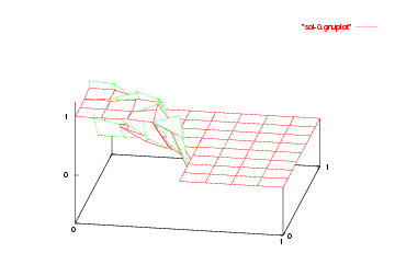
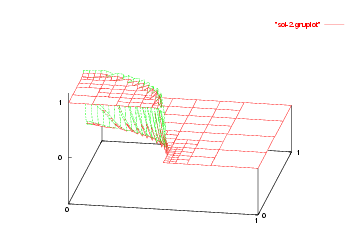
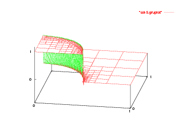
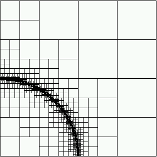
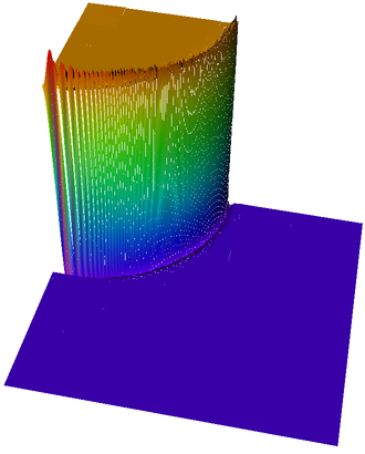
We show the solutions on the initial mesh, the mesh after two and after five adaptive refinement steps.


Then we show the final grid (after 5 refinement steps) and the solution again, this time with a nicer 3d rendering (obtained using the DataOutBase::write_vtk function and the VTK-based VisIt visualization program) that better shows the sharpness of the jump on the refined mesh and the over- and undershoots of the solution along the interface:


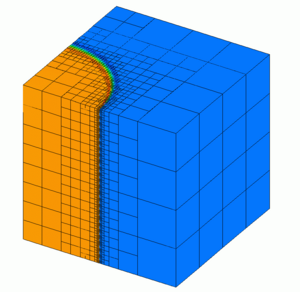
And finally we show a plot of a 3d computation.

Possibilities for extensions
For ideas for further extensions, please see see step-12.
The plain program
#include <iostream>
#include <fstream>
namespace Step12
{
template <int dim>
class BoundaryValues :
public Function<dim>
{
public:
BoundaryValues() = default;
virtual void value_list(
const std::vector<
Point<dim>> &points,
std::vector<double> & values,
const unsigned int component = 0) const override;
};
template <int dim>
void BoundaryValues<dim>::value_list(
const std::vector<
Point<dim>> &points,
std::vector<double> & values,
const unsigned int component) const
{
(void)component;
for (unsigned int i = 0; i < values.size(); ++i)
{
if (points[i](0) < 0.5)
values[i] = 1.;
else
values[i] = 0.;
}
}
template <int dim>
{
Assert(dim >= 2, ExcNotImplemented());
wind_field[0] = -p[1];
wind_field[1] = p[0];
wind_field /= wind_field.
norm();
return wind_field;
}
template <int dim>
class AdvectionProblem
{
public:
AdvectionProblem();
private:
void setup_system();
void assemble_system();
void refine_grid();
void output_results(const unsigned int cycle) const;
static void integrate_cell_term(DoFInfo &dinfo, CellInfo &info);
static void integrate_boundary_term(DoFInfo &dinfo, CellInfo &info);
static void integrate_face_term(DoFInfo & dinfo1,
DoFInfo & dinfo2,
CellInfo &info1,
CellInfo &info2);
};
template <int dim>
AdvectionProblem<dim>::AdvectionProblem()
: mapping()
, fe(1)
{}
template <int dim>
void AdvectionProblem<dim>::setup_system()
{
dof_handler.distribute_dofs(fe);
sparsity_pattern.copy_from(dsp);
system_matrix.reinit(sparsity_pattern);
solution.reinit(dof_handler.n_dofs());
right_hand_side.reinit(dof_handler.n_dofs());
}
template <int dim>
void AdvectionProblem<dim>::assemble_system()
{
const unsigned int n_gauss_points = dof_handler.get_fe().degree + 1;
n_gauss_points,
n_gauss_points);
assembler;
assembler.
initialize(system_matrix, right_hand_side);
dim,
dof_handler.begin_active(),
dof_handler.end(),
dof_info,
info_box,
&AdvectionProblem<dim>::integrate_cell_term,
&AdvectionProblem<dim>::integrate_boundary_term,
&AdvectionProblem<dim>::integrate_face_term,
assembler);
}
template <int dim>
void AdvectionProblem<dim>::integrate_cell_term(DoFInfo & dinfo,
CellInfo &info)
{
{
local_matrix(i, j) += -beta_at_q_point *
}
}
template <int dim>
void AdvectionProblem<dim>::integrate_boundary_term(DoFInfo & dinfo,
CellInfo &info)
{
const std::vector<Tensor<1, dim>> &normals =
static BoundaryValues<dim> boundary_function;
{
const double beta_dot_n =
if (beta_dot_n > 0)
local_matrix(i, j) += beta_dot_n *
else
local_vector(i) += -beta_dot_n *
}
}
template <int dim>
void AdvectionProblem<dim>::integrate_face_term(DoFInfo & dinfo1,
DoFInfo & dinfo2,
CellInfo &info1,
CellInfo &info2)
{
const unsigned int neighbor_dofs_per_cell =
const std::vector<Tensor<1, dim>> &normals =
{
const double beta_dot_n =
if (beta_dot_n > 0)
{
for (unsigned int i = 0; i < dofs_per_cell; ++i)
for (unsigned int j = 0; j < dofs_per_cell; ++j)
u1_v1_matrix(i, j) += beta_dot_n *
for (unsigned int k = 0; k < neighbor_dofs_per_cell; ++k)
for (unsigned int j = 0; j < dofs_per_cell; ++j)
u1_v2_matrix(k, j) +=
-beta_dot_n *
}
else
{
for (unsigned int i = 0; i < dofs_per_cell; ++i)
for (
unsigned int l = 0;
l < neighbor_dofs_per_cell; ++
l)
u2_v1_matrix(i, l) +=
beta_dot_n *
for (unsigned int k = 0; k < neighbor_dofs_per_cell; ++k)
for (
unsigned int l = 0;
l < neighbor_dofs_per_cell; ++
l)
u2_v2_matrix(k, l) +=
-beta_dot_n *
}
}
}
template <int dim>
{
preconditioner.
initialize(system_matrix, fe.n_dofs_per_cell());
solver.solve(system_matrix, solution, right_hand_side, preconditioner);
}
template <int dim>
void AdvectionProblem<dim>::refine_grid()
{
dof_handler,
solution,
gradient_indicator);
unsigned int cell_no = 0;
for (const auto &cell : dof_handler.active_cell_iterators())
gradient_indicator(cell_no++) *=
gradient_indicator,
0.3,
0.1);
}
template <int dim>
void AdvectionProblem<dim>::output_results(const unsigned int cycle) const
{
{
const std::string filename = "grid-" + std::to_string(cycle) + ".eps";
deallog <<
"Writing grid to <" << filename <<
'>' << std::endl;
std::ofstream eps_output(filename);
}
{
const std::string filename = "sol-" + std::to_string(cycle) + ".gnuplot";
deallog <<
"Writing solution to <" << filename <<
'>' << std::endl;
std::ofstream gnuplot_output(filename);
}
}
template <int dim>
void AdvectionProblem<dim>::run()
{
for (unsigned int cycle = 0; cycle < 6; ++cycle)
{
deallog <<
"Cycle " << cycle << std::endl;
if (cycle == 0)
{
}
else
refine_grid();
deallog <<
"Number of active cells: "
setup_system();
deallog <<
"Number of degrees of freedom: " << dof_handler.n_dofs()
<< std::endl;
assemble_system();
solve(solution);
output_results(cycle);
}
}
}
int main()
{
try
{
Step12::AdvectionProblem<2> dgmethod;
dgmethod.run();
}
catch (std::exception &exc)
{
std::cerr << std::endl
<< std::endl
<< "----------------------------------------------------"
<< std::endl;
std::cerr << "Exception on processing: " << std::endl
<< exc.what() << std::endl
<< "Aborting!" << std::endl
<< "----------------------------------------------------"
<< std::endl;
return 1;
}
catch (...)
{
std::cerr << std::endl
<< std::endl
<< "----------------------------------------------------"
<< std::endl;
std::cerr << "Unknown exception!" << std::endl
<< "Aborting!" << std::endl
<< "----------------------------------------------------"
<< std::endl;
return 1;
}
return 0;
}
void write_gnuplot(std::ostream &out) const
void add_data_vector(const VectorType &data, const std::vector< std::string > &names, const DataVectorType type=type_automatic, const std::vector< DataComponentInterpretation::DataComponentInterpretation > &data_component_interpretation={})
virtual void build_patches(const unsigned int n_subdivisions=0)
const std::vector< double > & get_JxW_values() const
const std::vector< Point< spacedim > > & get_quadrature_points() const
const Point< spacedim > & quadrature_point(const unsigned int q_point) const
const unsigned int n_quadrature_points
const std::vector< Tensor< 1, spacedim > > & get_normal_vectors() const
const Tensor< 1, spacedim > & shape_grad(const unsigned int i, const unsigned int q_point) const
const double & shape_value(const unsigned int i, const unsigned int q_point) const
void initialize(MatrixType &m, VectorType &rhs)
void initialize_update_flags(bool neighbor_geometry=false)
void initialize_gauss_quadrature(unsigned int n_cell_points, unsigned int n_boundary_points, unsigned int n_face_points, const bool force=true)
void initialize(const FiniteElement< dim, spacedim > &el, const Mapping< dim, spacedim > &mapping, const BlockInfo *block_info=nullptr)
void add_update_flags(const UpdateFlags flags, const bool cell=true, const bool boundary=true, const bool face=true, const bool neighbor=true)
void initialize(const MatrixType &A, const AdditionalData parameters)
Point< spacedim > point(const gp_Pnt &p, const double tolerance=1e-10)
Tensor< 2, dim, Number > l(const Tensor< 2, dim, Number > &F, const Tensor< 2, dim, Number > &dF_dt)
void run(const Iterator &begin, const std_cxx20::type_identity_t< Iterator > &end, Worker worker, Copier copier, const ScratchData &sample_scratch_data, const CopyData &sample_copy_data, const unsigned int queue_length, const unsigned int chunk_size)
::VectorizedArray< Number, width > pow(const ::VectorizedArray< Number, width > &, const Number p)


